Download
1 / 40
400 likes | 447 Views
Figure 13.1 Process of buying and selling a financial option. Figure 13.2 Profit from buying a call option on one share of Google stock. Figure 13.3 Profit from writing a call option on one share of Google stock.

E N D
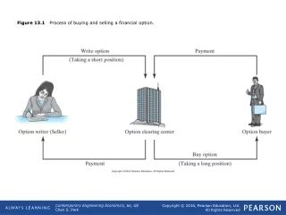
Figure 13.1 Process of buying and selling a financial option.
Figure 13.2 Profit from buying a call option on one share of Google stock.
Figure 13.3 Profit from writing a call option on one share of Google stock.
Figure 13.4 Profit from buying a put option on one share of Google stock.
Figure 13.5 Profit from writing a put option on one share of Google stock.
Table 13.1 Comparison Between Purchasing Stock versus Purchasing Options
Figure 13.6 Profit or loss as a function of the final stock price for each investment strategy.
Figure 13.7 Potential profit or loss with long position in a stock combined with long position in a put as a function of stock price at the expiration of option.
Figure 13.11 Creating a replicating portfolio by owning Δ shares of stock and b dollars worth of a risk-free asset such as a U.S. Treasury bond.
Figure 13.12 Risk-neutral probability approach to valuing an option.
Figure 13.13 Binomial lattice model with risk-neutral probabilities.
Figure 13.15 Two-period binomial lattice and option prices with the upper number at each node being the stock price and the lower number being the option price at that node.
Figure 13.16 The binominal representation of asset price over one year: (a) with only two changes in value, (b) with four changes in value, and (c) with daily changes in value.
Figure 13.17 Binomial lattice for Google stock for a period of four weeks.
Figure 13.18 Excel worksheet to evaluate the Black–Scholes formulas.
Figure 13.19 The analogy between a call option on a stock and a real option.
Figure 13.20 Definition of value of real-option, commonly known as “value of flexibility” or “real-option premium.”
Figure 13.21 Cash flow diagrams associated with demand scenarios in Example 13.8.
Figure 13.22 Types of real options.Source: “Get Real—Using Real Options in Security Analysis,” Frontiers of Finance, Volume 10, by Michael J. Mauboussin. Credit Suisse First Boston, June 23, 1999.
Figure 13.23 Transforming cash-flow data to obtain input parameters V0 and I2 for option valuation.
Figure 13.24 Cash flows associated with the two investment opportunities: a small-scale investment followed by a large-scale investment. The large-scale investment is contingent upon the small-scale investment.
Figure 13.25 Event tree: Lattice evolution of the underlying value of a project.
Figure 13.26 Decision tree diagram illustrating the process of reaching a decision at node ➌.
Figure 13.27 Decision tree for a scale-up option (valuation lattice).
Figure 13.28 The event tree that illustrates how the project’s value changes over time.
Figure 13.30 Sequential compound options (valuation lattice).
Figure 13.33 Sequential compound options (combined lattice).
Figure 13.34 Mathematical relationships between σ and σT. If Δ is small compared to 1, VT is log-normally distributed.
Figure 13.35 The process of obtaining the VT distribution by aggregating the periodic random cash-flow series. A risk simulation software such as Crystal Ball or @RISK may be used.