Download
1 / 32
330 likes | 477 Views
Thermal Transport in Nanostrucutures. Jian-Sheng Wang Center for Computational Science and Engineering and Department of Physics, NUS; IHPC & SMA. Outline. Heat transport using classical molecular dynamics

E N D
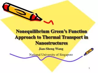
Thermal Transport in Nanostrucutures Jian-Sheng Wang Center for Computational Science and Engineering and Department of Physics, NUS; IHPC & SMA
Outline • Heat transport using classical molecular dynamics • Nonequilibrium Green’s function (NEGF) approach to thermal transport, ballistic and nonlinear • QMD – classical molecular dynamics with quantum baths • Outlook and conclusion
Fourier’s Law of Heat Conduction Fourier proposed the law of heat conduction in materials as J = - κT where J is heat current density, κ is thermal conductivity, and T is temperature. Fourier, Jean Baptiste Joseph, Baron (1768 – 1830)
Normal & Anomalous Heat Transport 3D bulk systems obey Fourier’s law (insulating crystal: Peierls’ theory of Umklapp scattering process of phonons; gas: kinetic theory, κ = 1/3 cvl ) In 1D systems, variety of results are obtained and still controversial. See S Lepri et al, Phys Rep 377, 1 (2003); A Dhar, arXiv:0808.3256, for reviews. TL TH J
Carbon Nanotubes Heat conductivity of carbon nanotubes at T = 300K by nonequilibrium molecular dynamics. From S Maruyama, “Microscale Thermophysics Engineering”, 7, 41 (2003). See also Z Yao at al cond-mat/0402616, G Zhang and B Li, cond-mat/0403393.
A Chain Model for Heat Conduction ri= (xi,yi) TR TL Φi m Transverse degrees of freedom introduced
Nonequilibrium Molecular Dynamics • Nosé-Hoover thermostats at the ends at temperature TL and TR • Compute steady-state heat current: j =(1/N)Si d (eiri)/dt, where ei is local energy associated with particle i • Define thermal conductivity k by <j> = k (TR-TL)/(Na) N is number of particles, a is lattice spacing.
slope=1/3 Conductivity vs size N Model parameters (KΦ, TL, TR): Set F (1, 5, 7), B (1, 0.2, 0.4), E (0.3, 0.3, 0.5), H (0, 0.3, 0.5), J (0.05, 0.1, 0.2) , m=1, a=2, Kr=1. From J-S Wang & B Li, Phys Rev Lett 92, 074302 (2004). slope=2/5 ln N
Nonequilibrium Green’s Function Approach Tfor matrix transpose mass m = 1, ħ = 1 Left Lead, TL Right Lead, TR Junction Part
Heat Current Where G is the Green’s function for the junction part, ΣL is self-energy due to the left lead, and gL is the (surface) Green’s function of the left lead.
Landauer/Caroli Formula • In systems without nonlinear interaction the heat current formula reduces to that of Laudauer formula: See, e.g., Mingo & Yang, PRB 68, 245406 (2003); JSW, Wang, & Lü, Eur. Phys. J. B, 62, 381 (2008).
Contour-Ordered Green’s Functions τ complex plane See Keldysh, or Meir & Wingreen, or Haug & Jauho
Adiabatic Switch-on of Interactions Governing Hamiltonians HL+HC+HR +V +Hn HL+HC+HR +V G HL+HC+HR Green’s functions G0 g t = − Equilibrium at Tα t = 0 Nonequilibrium steady state established
Feynman Diagrams Each long line corresponds to a propagator G0; each vertex is associated with the interaction strength Tijk.
Leading Order Nonlinear Self-Energy σ = ±1, indices j, k, l, … run over particles
Energy Transmissions The transmissions in a one-unit-cell carbon nanotube junction of (8,0) at 300 Kelvin. From JSW, J Wang, N Zeng, Phys. Rev. B 74, 033408 (2006).
Thermal Conductance of Nanotube Junction Cond-mat/0605028
Molecular Dynamics Molecular dynamics (MD) for thermal transport Equilibrium ensemble, using Green-Kubo formula Non-equilibrium simulation Nosé-Hoover heat-bath Langevin heat-bath Disadvantage of classical MD Purely classical statistics Heat capacity is quantum below Debye temperature of 1000 K Ballistic transport for small systems is quantum
Quantum Corrections • Methods due to Wang, Chan, & Ho, PRB 42, 11276 (1990); Lee, Biswas, Soukoulis, et al, PRB 43, 6573 (1991). • Compute an equivalent “quantum” temperature by • Scale the thermal conductivity by (1) (2)
Quantum Heat-Bath & MD • Consider a junction system with left and right harmonic leads at equilibrium temperatures TL & TR, the Heisenberg equations of motion are • The equations for leads can be solved, given (3) (4)
Quantum Langevin Equation for Center • Eliminating the lead variables, we get where retarded self-energy and “random noise” terms are given as (5) (6)
Properties of Quantum Noise (7) (8) (9) For NEGF notations, see JSW, Wang, & Lü, Eur. Phys. J. B, 62, 381 (2008).
Quasi-Classical Approximation, Schmid (1982) • Replace operators uC & by ordinary numbers • Using the quantum correlation, iħ∑> or iħ∑< or their linear combination, for the correlation matrix of . • Since the approximation ignores the non-commutative nature of , quasi-classical approximation is to assume, ∑> = ∑<. • For linear systems, quasi-classical approximation turns out exact! See, e.g., Dhar & Roy, J. Stat. Phys. 125, 805 (2006).
Implementation • Generate noise using fast Fourier transform • Solve the differential equation using velocity Verlet • Perform the integration using a simple rectangular rule • Compute energy current by (10) (11)
Comparison of QMD with NEGF Three-atom junction with cubic nonlinearity (FPU-). From JSW, Wang, Zeng, PRB 74, 033408 (2006) & JSW, Wang, Lü, Eur. Phys. J. B, 62, 381 (2008). QMD ballistic QMD nonlinear kL=1.56 kC=1.38, t=1.8 kR=1.44
From Ballistic to Diffusive Transport 1D chain with quartic onsite nonlinearity (Φ4 model). The numbers indicate the length of the chains. From JSW, PRL 99, 160601 (2007). Classical, ħ 0 4 16 NEGF, N=4 & 32 64 256 1024 4096
Electron Transport & Phonons • For electrons in the tight-binding form interacting with phonons, the quantum Langevin equations are (12) (13) (14) (15)
Ballistic to Diffusive Electronic conductance vs center junction size L. Electron-phonon interaction strength is m=0.1 eV. From Lü & JSW, arXiv:0803.0368.
Conclusion & Outlook • MD is useful for high temperature thermal transport but breaks down below Debye temperatures • NEGF is elegant and efficient for ballistic transport. More work need to be done for nonlinear interactions • QMD for phonons is correct in the ballistic limit and high-temperature classical limit. Much large systems can be simulated (comparing to NEGF)
Baowen Li Pawel Keblinski Jian Wang Jingtao Lü Nan Zeng Lifa Zhang Xiaoxi Ni Eduardo Cuansing Jinwu Jiang Saikong Chin Chee Kwan Gan Jinghua Lan Yong Xu Collaborators