Download
1 / 52
830 likes | 2.01k Views
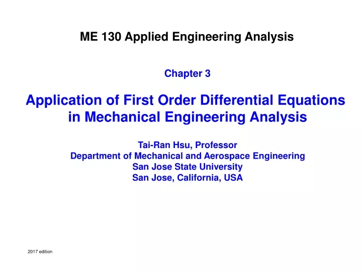
ME 130 Applied Engineering Analysis. Chapter 3 Application of First Order Differential Equations in Mechanical Engineering Analysis Tai-Ran Hsu, Professor Department of Mechanical and Aerospace Engineering San Jose State University San Jose, California, USA. 2017 edition.

E N D
ME 130 Applied Engineering Analysis Chapter 3 Application of First Order Differential Equations in Mechanical Engineering Analysis Tai-Ran Hsu, Professor Department of Mechanical and Aerospace Engineering San Jose State University San Jose, California, USA 2017 edition
Chapter Learning Objectives 1. Learn to solve typical first order ordinary differential equations of both homogeneous and non-homogeneous types with and without specified conditions. 2. Learn the definitions of essential physical quantities in fluid mechanics analyses. 3. Learn the Bernoulli’s equation relating to the driving pressure and the velocities of fluids in motion. 4. Learn to use the Bernoulli’s equation to derive differential equations describing the flow of non-compressible fluids in large tanks and funnels of different geometry. 5. Learn to find time required to drain liquids from containers of given geometry and dimensions. 7. Learn how to derive differential equations to predict required times to heat or cool solids by surrounding fluids. 8. Learn to derive differential equations describing the motion of rigid bodies under the influence of gravitation. 6. Learn the Fourier law of heat conduction in solids and Newton’s cooling law for convective heat transfer in fluids.
Part 1 Review of Solution Methods for First Order Differential Equations In “real-world,” there are many physical quantities that can be represented by functions involving only one of the four independent variables e.g., (x, y, z, t) Equations involving highest order derivatives of order one = 1st order differential equations Examples: Function σ(x)= the stress in a uni-axial stretched metal rod with tapered cross section (Fig. a), or Function v(x)=the velocity of fluid flowing in a straight channel with varying cross-section (Fig. b): Fig. b P1>P2 Fig. a v(x) x σ(x), Δ(x) P1 P2 x Mathematical modeling using differential equations involving these functions are classified as First Order Differential Equations
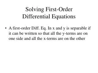
“Separable” ordinary ODEs The solution of the following DE = u(x): (3.1) can be obtained by re-arranging the terms as: h(u) du = g(x)dx We notice that the new form of the original equation now has: The Left-Hand-Side (LHS) = function of u (or constants) only, and the Right-Hand-Side (RHS) = function of the variable x (or constants) only. We have thus effectively “separated” the function u and the variable x on either sides of the equation. This separation has lead to the following solution of u(x) by integrating both sides to obtain: (3.2) where c = integration constant SELF-learning: Example 3.1 Often, the DE is not separable as in Equation (3.1). In such cases, we need to derive Solution method for First order DEs by the following methods.
General Solution Methods for First Order ODEs A. Solution of linear homogeneous equations (p.61): Typical form of the First order ordinary differential equation: (3.3) It is called the FIRST ORDER ordinary differential equation because the highest order of derivative appears in the equation is of order ONE. The equation is called homogeneous because the RHS of the DE is ZERO. The solution u(x) in Equation (3.3) is: (3.4) where K = constant to be determined by given condition, and the function F(x) has the form: (3.5) in which the function p(x) is given in the differential equation in Equation (3.3)
Example 3.2(P.62): Given DE: We have: p(x) = -Sin x as in Equation (3.3), which leads top(x)dx = Cos x and hence from Equation (3.5) we have The solution of the ordinary differential equation (ODE) in Equation (a) is available in Equation (3.4), or in the form: where K = arbitrary constant
B. Solution of linear Non-homogeneous equations (P.62): Typical differential equation: (3.6) The appearance of function g(x) in Equation (3.6) makes the DE to be non-homogeneous The solution of ODE in Equation (3.6) is similar to the solution of homogeneous equation in a little more complex form than that for the homogeneous equation in (3.3): (3.7) where function F(x) can be obtained from Equation (3.5) as: (3.5)
Example 3.2 Solve the following differential equation (p. 57): (a) but with a prescribed condition u(0) = 2 Solution: By comparing terms in Equation (a) and (3.6), we have: p(x) = -sin x and g(x) = 0. Thus by using Equation (3.7), we have the solution: , leading to the solution: in which the function F(x) is: Since the given condition is u(0) = 2, we have: , or K = 5.4366. Hence the solution of Equation (a) is: u(x) = 5.4366 e-Cos x
Example 3.4: solve the following differential equation (p. 59): (a) (b) with the condition: u(0) = 2 Solution: By comparing the terms in Equation (a) and those in Equation (3.6), we will have: p(x) = 2 and g(x) = 2, which leads to: By using the solution given in Equation (3.7), we have: We will use the condition given in (b) to determine the constant K: Hence, the solution of Equation (a) with the condition in (b) is:
Part 2 Application of First Order Differential Equation to Fluid Mechanics Analysis (P.64)
Fundamental Principles of Fluid Mechanics Analysis - A substance with mass but no shape Fluids Compressible (Gases) Non-compressible (Liquids) Moving of a fluid requires: ● A conduit, e.g., tubes, pipes, channels ● Driving pressure, or by gravitation, i.e., difference in “head” ● Fluid flows with a velocity v from higher pressure (or elevation) to lower pressure (or elevation) ● Fluid flows from higher elevation to low elevation • Derived from the law of conservation of mass • It relates the flow velocity (v) and the cross-sectional area (A) The law of continuity The rate of volumetric flow follows the rule: q = A1v1 = A2v2 m3/s
Common Terminologies in Fluid Mechanics Analysis Higher pressure (or elevation) The total mass flow, (3.8a) (3.8b) Total mass flow rate, Total volumetric flow rate, (3.8c) Total volumetric flow, (3.8d) in which ρ = mass density of fluid (g/m3), A = cross-sectional area (m2), v = velocity (m/s), and Δt = duration of flow (s). The units associated with the above quantities are (g) for grams, (m) for meters and (sec) for seconds. ● In case the velocity varies with time, i.e., v = v(t): Then the change of volumetric flow becomes: ∆V = A v(t) ∆t, with ∆t = time duration for the fluid flow (3.9)
The Bernoullis Equation (The mathematical expression of the law of physics relating the driving pressure and velocity in a moving non-compressible fluid) Flow Path Using the Law of conservation of energy, or the First Law of Thermodynamics, for the energies of the fluid at State 1 and State 2, we can derive the following expression relating driving pressure (p) and the resultant velocity of the flow (v): The Bernoullis Equation:
Application of Bernoullis equation in liquid (water) flow in a LARGE reservoir (p.66): State 1 Large Reservoir Water tank Tap exit State 2 Tap exit From the Bernoullis’s equation, we have: (3.10) If the difference of elevations between State 1 and 2 is not too large, we can have: p1≈ p2 Also, because it is a LARGE reservoir (or tank), we realize that v1 << v2, or v1≈ 0 Equation (3.10) can be reduced to the form: from which, we may express the exit velocity of the liquid at the tap v2 to be: (3.11)
Application of 1st Order DE in Drainage of a Water Tank (p.62) Tap Exit The physical condition for math modeling: The law of conservation of mass: The total volume of water leaving the tank during ∆t: (∆Vexit) = The total volume of water supplied by the tank during ∆t: (∆Vtank) We have from Equation (3.9): ∆V = A v(t) ∆t, in which v(t) is the velocity of moving fluid Thus, the volume of water leaving the tap exit is: (a) with given in Equation (3.11)
Next, we need to formulate the water supplied by the tank, ∆Vtank: The initial water level in the tank is ho The water level keeps dropping after the tap exit is opened, and the reduction of Water level is CONTINUOUS Let the water level at time t be h(t) We let ∆h(t) = amount of drop of water level during time increment ∆t Then, the volume of water LOSS in the tank is: (b) (Caution: a “-” sign is given to ∆Vtank b/c of the LOSS of water volume with increasing time during ∆t) The total volume of water leaving the tank during ∆t (∆Vexit) in Equation (a) = The total volume of water supplied by the tank during ∆t (∆Vtank) in Equation (b): Equation (a): Equation (b): (c) (d) By re-arranging the above:
If the process of draining is indeed CONTINUOUS, i.e., ∆t → 0, we will have Equation (d) expressed in the “differential” rather than “difference” form as follows: (3.13) (f) with an initial condition of h(0) = ho Equation (3.13) is the 1st order differential equation for the CONTINUOUS draining of a water tank. The solution of Equation (3.13) can be obtained by separating the function h(t) and the variable t by re-arranging the terms in Equation (3.13) in the following way: Upon integrating on both sides: where c = integration constant from which, we obtain the solution of Equation (3.13) to be: The constant is determined from the initial condition in Equation (f). The complete solution of Equation (3.13) with the initial condition in Equation (f) is thus: (g)
The solution in Equation (g) will allow us to determine the water level in the tank at any given instant, t. One may imagine that PHYSICALLY, the time required to drain the tank is the time te. Mathematically, it can be expressed as h(te) = 0: We may solve the above algebraic expression for te to be: Numerical example (P.70): Tank diameter, D = 12” = 1 ft. Drain pipe diameter, d = 1” = 1/12 ft. Initial water level in the tank, ho = 12” = 1 ft. Gravitational acceleration, g = 32.2 ft/sec. The time required to empty the tank is: So, now you know how to determine the time required to drain a ”fish tank” a “process tank” or a “swimming pool,” Make sure you do.
Application of 1st Order DE in Drainage of Tapered Funnels (p.71) Tapered funnels are common piece of equipment used in many process plants, e.g., in wine bottling: Diameter D Design of tapered funnels involves the determination of configurations, i.e. the tapered angle ϴ, and the diameters D and lengths of sections of the funnel (a, b and c) for the intended liquid content. It is also required the determination on the time required to empty the contained liquid. a θ b c
Formulations on Water of Liquid Level in Tapered Funnels The physical solution we are seeking is the water level at ANY given time t, y(t) after the water is let to flow from the exit of the funnel at t = 0+. θ The “real” funnel has an outline of frustum cone with smaller circular opening in the end “A” allowing water to flow. In the subsequent analysis, we assume that the funnel has an outline shape of “right cone” with its tip at “O” instead Initial water level H y(t) A Small (negligible) o Funnel opening diameter d We assume the initial water level in the funnel = H Once the funnel exit is open, and water begin to flow, the water level in the funnel at given time t is represented by the function y(t). Funnel exit We will use the same principle to formulate the expression for y(t) for the straight tank: The total volume of water leaving the funnel during ∆t: (∆Vexit)= The total volume of water supplied by the funnel during ∆t: (∆Vfunnel)
Determine the Instantaneous Water Level in a Tapered Funnel, y(t): The total volume of water leaving the tank during ∆t: (∆Vexit) = (Aexit) (ve) (∆t) Drop water level θ A VERY THIN H2O disk with radius r(y), thickness Δy But from Equation (3.11), we have the exit velocity ve to be: r(y) Initial water level H -∆y y(t) which leads to: A Small (a) o Funnel opening diameter d The total volume of water supplied by the tank during ∆t: ∆Vfunnel = volume of the cross-hatched in the diagram Funnel exit velocity ve ∆Vfunnel =- [π (r(y)2] (∆y) y (b) A “-ve” sign to indicate decreasing ∆Vfunnel with increasing y(t) r(y) (c) From the diagram in the left, we have: Hence by equating (a) and (b) with r(y) given in (c), we have: θ y(t) (d) For a CONTINUOUS variation of y(t), we have ∆t→0, we will have the differential equation for y(t) as: o (e)
Numerical Example on the Drainage of a Tapered Funnel (p. 68): To determine the time required to empty the funnel with initial water level of 150 mm and with the dimensions shown in the figure. ● This is a special case of the derivation of a general tapered funnel with θ = 45o. ● We thus have the differential equation similar to Equation (e) in the last slide with tanθ = tan45o = 1: (a) (b) with condition: Equation (a) is a 1st order DE, and its solution is obtained by integrating both sides w.r.t variable t: (c) The integration constant c is determined by using Equation (b) → c = 2H5/2/5, which leads to the complete solution of : (d) If we let time required to empty (drain) the funnel to be te with y(te) = 0, we will solve Equation (e) With these conditions to be: (e)
Example on the drainage of a funnel in a winery: To design a funnel that will fill a wine bottle of given geometry and dimensions. Design objective: To provide SHORTEST time in draining the funnel for fastest bottling process Given ? ? Max space given Diameter Given ? Bottle with given Geometry and Dimensions (such as in Example 2.9 on P. 36) Refer to Problem 3.15 on p. 96
Part 3 Applications of First Order Differential Equations to Heat Transfer Analysis The Three Modes of Heat Transmission: ●Heat conduction in solids ● Heat convection in fluids ● Radiation of heat in space
Review of Fourier Law for Heat Conduction in Solids ●Heat flows in SOLIDS by conduction ● Heat flows from the part of solid at higher temperature to the part at lower temperature - a situation similar to water flows from higher elevation to lower elevation ● Thus, there is definite relationship between heat flow (Q) and the temperature difference (∆T) in the solid ●Relating the Q and ∆T is what the Fourier law of heat conduction is all about Derivation of Fourier Law of Heat Conduction: A solid slab: With the left surface maintained at temperature Ta and the right surface at Tb Heat will flow from the left to the right surface if Ta > Tb where Ta= temp. at left face, Tb = temp. at right face Tb By logics & observations, we can formulate the total amount of heat flow (Q) From the left face to the right face is proportional to the following: Ta where A = the area of the solid faces to which heat flows; t = time allowing heat flow; and d = the distance of heat flow Replacing the sign in the above expression by adding a constant k, leads to: (3.17) The constant k in Equation (3.17) is “thermal conductivity” – treated as a property of the solid material with a unit: Btu/in-s-oF of W/m-oC. Physically, k is a measure of how “easy” is the material for allowing Heat to flow through. K is constant for common engineering materials in “normal” temperature ranges.
The amount of total heat flow in a solid as expressed in Equation (3.14) is useful, but make less engineering sense without specifying the area A and time t in the heat transmission process. Consequently, the term “Heat flux” (q) – a sense of the intensity of heat conduction is used more frequently in engineering analyses. From Equation (3.17), we may define the heat flux as: (3.18) with a unit of: Btu/in2-s, or W/cm2 We realize Equation (3.18) is derived from a situation of heat flow through a thickness of a slab with specified temperatures at both surfaces. The temperature variation withinthe solid often is needed in engineering analysis. Recognize that this variation is CONTINUOUS. So we may express it by function T(x) with x being the variable that determine the value of the function T(x). The corresponding heat flux within the solid in this case can be expressed by the following derivation: By following the expression in Equation (3.18), we will have the heat flux to be: (3.19) B/C function T(x) is a CONTINUOUS varying function w.r.t variable x, (meaning ∆x→0), We will have the following from Equation (2.1): (3.20) Equation (3.20) is the mathematical expression of Fourier Law of Heat Conduction in the x-direction
Example 3.7 (p. 77): A metal rod has a cross-sectional area 1200 mm2 and 2m in length. It is thermally insulated in its circumference, with one end being in contact with a heat source supplying heat at 10 kW, and the other end maintained at 50oC. Determine the temperature distribution in the rod, if the thermal conductivity of the rod material is k = 100 kW/m-oC. Solution: The total heat flow Q per unit time t(Q/t) in the rod is given by the heat source to the left end, i.e. 10 kW. Because heat flux is q = Q/(At) as shown in Equation (3.18), we have (Q/t) = qA = 10 kW as in Equation (3.20), we thus have: But the Fourier Law of heat conduction requires (a) (b) Expression in (a) is a 1st order differential equation, and its solution is: T(x) = -83.33x + c If we use the condition: T(2) = 50oC, we will find c = 216.67, which leads to the complete solution:
Heat Flux in Space Expressions in 3-dimensional form We recognize that: ● Heat flows in the direction of decreasing temperature in a solid ● In solids with temperature variations in all direction, heat will flow in ALL directions ● So, in general, there can be 3-dimensional heat flow in solids ● This leads to 3-dimensional formulation of heat flux ● Heat flux q(r,t) is a vector quantity, with r = position vector, representing (x, y, z) The magnitude of vector q(r,t) is: (3.24) with the components of q(x,y,z,t) along respective x-, y- and z-coordinates: In general, the heat flux vector in the Fourier Law of heat conduction can be expressed as: (3.23) q(r,t) = -kT(r,t)
Examples of Heat Flux in a 2-D Plane Tubes with longitudinal fins are common in many heat exchangers and boilers tubes for effective heat exchange between the hot fluids inside the tube to cooler fluids outside: The heat inside the tube flows along the square (plate)-fins to the cool contacting fluid outside. Extened solid heat flow surface will facilitate more heat flow from inside The tubes to the outside cooler fluids. So, it is desirable to analyze how effective heat can flow in the cross-section of the fin. Cool HOT Fins are also used to conduct heat from the hot gas inside the cylinder of an Internal combustion engine to the outside cooling air in motorcycles: Cold Cooling fins Hot Cross-section of a tube with longitudinal fins with only one fin shown
Heat Flux in a 2-D Plane is also common in electronics devices for cooling heat generating ICs inside the packages. Typical Heat Spreaders in Microelectronics Cooling: Heat spreader of common cross-sections Heat dissipation to the surrounding cool air or liquid Heat flow in a 2-dimensional plane, by Fourier Law in x-y plane q q q Heat Source e.g., IC chip
PROPER FORMS OF Fourier Law of Heat Conduction in 2-Dimensions For one-dimensional heat flow: Heat flow Heat flow +x T(x) +X T(x) X=0 X=0 NOTE: The correct sign attached to q(x) changes with the change of direction of heat flow!! For two-dimensional heat flow: y q –heat flux in or out in the solid plane qy Change of sign in the General form of Fourier Law of Heat Conduction: qx q(r,t) = ±kT(r,t) Temp: T(x,y) x Question: How to assign the CORRECT sign in heat flux??
Sign of Heat Flux – follows Hsu’s convention: With know heat flow directions: q – heat flux in or out in the solid plane; Outward NORMAL (n) (+VE) y qy ●OUTWARD NORMAL = Normal line pointing AWAY from the solid surface qx Temp: T(x,y) x
Example 3.8: Express the heat flux across the four edges of a rectangular block with correct +ve or –ve sign (p.80) with temp. distribution in the solid plane being T(x,y) y q3 The direction of heat fluxes is prescribed. Thermal conductivity of the material k is given. Given temp. T(x,y) q1 q2 q4 x Solution: Use the Hsu sign convention:
Example 3.9 Heat fluxes leaving a heat spreader of half-triangular cross-section. (p.81) Heat flow in the Spreader: A Ambient temp. = 20oC A Heat Spreader Given: T(x,y) = 100 + 5xy2 – 3x2y oC 4 cm T(x,y) Thermal conductivity k = 0.021 W/cm-oC T(x,y) B c B C 2 cm IC-Chip: Heat Source Solution: Set coordinate system and Identify outward normals: y A qAC qAB -nx x B C -ny qBC
A. Heat flux across surface BC: The direction of heat flow is known (from heat source to the spreader) -ve n Case 3 or 4; qBC is not along n Case 4 with –ve sign B. Heat flux across surface AB: We need to verify the direction of heat flow across this surface first:: Checking the temperature at the two terminal points of the Edge AB: At Point B (x = 0 and y = 0) the corresponding temperature is: The same temperature at terminal A So, heat flows from the spreader to the surrounding. y It is Case 3 in Fourier law, we thus have: A -nx qab T(x,y) B C x
C. Heat flux across surface AC: Surface AC is an inclined surface, so we have a situation as illustrated below. Use the same technique as in Case B, we may find the temperature at both terminal A and C to be 100oC > 20oC in ambient. So heat leaves the surface AC to the ambient. y +ny qac,y A Based on the direction of the components of the heat flow and outward normal, we recognize Case 1 for both qac,x and qac,y. Thus we have: qac +nx qac,x x B C and The heat flux across the mid-point of surface AC at x = 1 cm and y = 2 cm is:
Review of Newton’s Cooling Law for Heat Convection in Fluids ● Heat flow (transmission) in fluid by CONVECTION ● Heat flow from higher temperature to low temperature in fluids ● Motion of fluids causes heat convection ● As a rule-of-thumb, the amount of heat transmission by convection is proportional to the velocity of the moving fluid Mathematical expression of heat convection – The Newton’s Cooling Law A fluid of non-uniform temperature in a container: Heat flows from Ta to Tb with Ta > Tb. The heat flux between A and B can be expressed by: (3.25) where h = heat transfer coefficient (W/m2-oC) The heat transfer coefficient h in Equation (3.25) is normally determined by empirical expression, with its values relating to the Reynolds number (Re) of the moving fluid. The Reynolds number is expressed as: with ρ = mass density of the fluid; L = characteristic length of the fluid flow, e.g., the diameter of a circular pipe, or the length of a flat plate; v = velocity of the moving fluid; μ = dynamic viscosity of the fluid
Heat Transfer in Solids Submerged in Fluids ●There are numerous examples in REALITY of which solids are in contact with fluids at different temperatures: Refrigeration: Heat Treatment: Cool Enclosure Hot Enclosure Cool Solid Hot Solid q T(r,t) q T(r,t) Bulk Fluid Temp: Tf Bulk Fluid Temp: Tf ● In such cases, there is heat flow between the contacting solid and fluid. ● But the physical laws governing heat flow in solids is the Fourier Law and that in fluids by the Newton’s Cooling Law So, mathematical modeling for the contacting surface in this situation requires the use of bothFourier Law and Newton’s Cooling Law: Mathematical Modeling of Small Solids in Refrigeration and Heating: We will formulate a simplified case with assumptionson: ● the solid is initially at temperature To ● the solid is so small that it has uniform temperature THROUGHOUT, but its temperature varies with time t , i.e., T = T(t) ● the time t begins at the instant at which the solid is submerged in the fluid at a different temperature Tf ● variation of temp. in the solid is attributed by the heat supplied, or removed by the fluid
Derivation of Math Model for Heat Transfer in Solids Submerged in Fluids The solid is small, so the surface temperature Ts(t) = T(t), the solid temperature Bulk Fluid Solid Temp T(t) Bulk Fluid Temp Tf q Heat flows in the fluid, when T(t) ≠ Tf, the bulk fluid temp. Ts(t) Heat flows in the fluid follows the Newton Cooling Law expressed in Equation (3.25), i.e.: (3.26) q = h [Ts(t) – Tf] = h [T(t) – Tf] where h = heat transfer coefficient between the solid and the bulk fluid From the First Law of Thermodynamics, the heat required to produce temperature change in a solid ∆T(t) during time period ∆t can be obtained by the following physical relationship: Change in internal energy of the small solid during ∆t Net heat flow from the small solid to the surrounding fluid during ∆t = Q = q As∆t = h As[ T(t) – Tf ] ∆t - ρcV ∆T(t) = (b) where ρ = mass density of the solid; c = specific heats of solid V = volume of the solid; As = contacting surface between the solid and bulk fluid
From Equation (b), we express the rate of temperature change in the solid to be: (c) Since h , ρ, c and V on the right-hand-side of Equation (c) are constant, we may lump these three constants to let: (3.27) with a unit (/m2-s) (3.27) Equation (c) is thus expressed as: Since the change of the temperature of the submerged solid T(t) is CONTINOUSwith respect to time t, i.e., , and if we replace the contact surface area As to a generic symbol A, we can express Equation (3.27) in the form of a 1st order differential equation: (3.27) with an initial condition: (3.27a)
Example 3.10:Determine the time required to cool down a solid object initially at 80oC to 8oC. It is placed in a refrigerator with its interior air maintained at 5oC. If the coefficient α = 0.002/m2-s and the contact area between the solid and the cool air in the refrigerator is A = 0.2 m2. Solution: We have To = 80oC, Tf = 5oC, α = 0.002/m2-s and A = 0.2 m2 Substituting the above into Equation (3.23) will lead to the following 1st order differential equation: (a) (b) with the condition: T(0) = 80oC (c) Equation (a) can be re-written as: (d) Integrating both sides of Equation (c): (e) Leads to the solution: The integration constant c in Equation (e) can be obtained by the condition T(0) = 80oC in Equation (b) with c = 75. consequently, the solution T(t) is: (f) If te = required time for the solid to drop its temperature from 80oC to 8oC, we should have: (g) Solve Equation (g) for te = 8047 s or 2.24 h What would you do if the required time to cool down the solid is too long?
Part 4 Applications of First Order Differential Equations to Kinematic Analysis of Rigid Body Dynamics We will demonstrate the application of 1st order differential equation in rigid body dynamics using Newton’s Second Law ∑F = ma
Rigid Body Motion Under Influence of Gravitation: There are many engineering systems that involve dynamic behavior under strong influence of gravitation. Examples such as: Rocket launch The helicopter The paratroopers
A Rigid Body in Vertical Motion Under Influence of Gravitation X Free Fall Thrown-up (acceleration by gravitation) (Deceleration by Gravitation) Galileo Galilei Velocity v(t) Velocity v(t) F(t) F(t) R(t) R(t) Math W W Modeling X = 0 Solution sought: ● The instantaneous position x(t) ● The instantaneous velocity v(t) ● The maximum height the body can reach, and the required time with initial velocity vo in the “thrown-up” situation Galileo’s free-fall experiment from the leaning tower in Pisa, Italy, December 1612 These solutions can be obtained by first deriving the mathematical expression (a differential equation in this case), and solve for the solutions By kinematics of a moving solid: If the instantaneous position of the solid is expressed as x(t), we will have: to be the instantaneous velocity, and to be the instantaneous acceleration (or deceleration)
Derivation of Math Expression for Free-Fall of a Solid: X Fall-down Thrown-up Referring to the Left-half of the diagram: Velocity v(t) Velocity v(t) Forces acting on the falling solid at time t include: F(t) F(t) R(t) R(t) W = the weight R(t) = the resistance of the air on the falling solid F(t) = the dynamic (inertia) force due to changing velocity of the fall under gravitational acceleration (g) W W X = 0 • The weight of the body, w = mg, in which m = mass of the body, and g = gravitational acceleration (g = 9.81 m/s2). This force always points towards the Earth. (2) The resistance encountered by the moving body in the medium such as air, R(t) = c v(t), in which c is the proportional constant determined by experiments and v(t) is the instantaneous velocity of the moving body. R(t) act opposite to the direction of motion. (3) The dynamic (or inertia) force, F(t) = ma(t), in which a(t) is the acceleration (or deceleration with a negative sign) of the solid at time t – the Newton’s Second Law One should notice that F(t) carries a sign that is opposite to the acceleration (Tell me your personal experience??)
Case A: Free-Fall of a solid: X Fall-down The forces acting on the falling solid should be in equilibrium at time t: Velocity v(t) By using a sign convention of forces along +ve x-axis being +ve, we have: F(t) R(t) ∑ Fx = 0 W Leads to: ∑ Fx = -W + R(t) + F(t) = 0 which yields to the following 1st order differential equation: (3.28) with an initial condition: (a)
Case B: Throw-up of a solid with initial velocity vo: As in the case of “Free-fall,” the forces acting on the Up-moving solid should be in equilibrium at time t: X Thrown-up By using a sign convention of forces along +ve x-axis Being +ve for the forces, we have: Velocity v(t) F(t) ∑ Fx = 0 R(t) Leads to: ∑ Fx = -W - R(t) - F(t) = 0 W with W = mg, R(t) = cv(t), and X = 0 A 1st order differential equation is obtained: (3.25) with an initial condition: (a)
The solution of Equation (3.25) is obtained by comparing it with the typical 1st order differential equation in Equation (3.6) with solution in Equation (3.7): (3.6) (3.7) with a solution: The present case has: , Consequently, the solution of Equation (3.25) has the form: (3.29) In which the constant K is determined by the given initial condition in Equation (a), with: (b) The complete solution of Equation (3.25) with the substitution of K in Equation (b) into Equation (3.26): (3.30)
The instantaneous position of the rigid body at time t can be obtained by: where the velocity function v(t) is given in Equation (3.29) The time required for the rigid body to reach the maximum height tm is the time at which The upward velocity of the body reduced to zero. Mathematically, it is expressed as: v(tm) = 0 in Equation (3.30): Solve tm from the above equation, resulting in: (3.31)
Example 3.10 An armed paratrooper with ammunitions weighing 322 lbs jumped with initial velocity from an airplane at an attitude of 10,000 feet with negligible side wind. Assume the air resistance R(t) the paratrooper encountered with is: R(t)= c[V(t)]2 in which the coefficient c = 15. Determine: • The appropriate equation for the instantaneous descending velocity of the paratrooper, and (b) The function of the descending velocity v(t) • The time required to land • The impact velocity upon landing Solution: (a) Differential equation for the velocity v(t): The total mass of the falling body, m = 322/32.2 = 10 slug, and the air resistance, R(t) = cv(t) = 15[v(t)]2 The instantaneous descending velocity, v(t) can be obtained by using Equation (3.29) as: (a) (b) or in another form: (c) with the condition: v(0) = o (b) The solution of Equation (b) with the condition in Equation (c) is: (d) (Refer to P. 88 of the printed notes for procedure to the above solution)