Chapter 2 Differential Equations of First Order

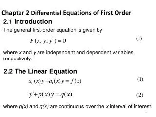
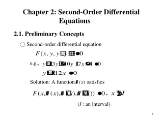
1. 2.1 Introduction The general first-order equation is given by where x and y are independent and dependent variables, respectively. Chapter 2 Differential Equations of First Order 2.2 The Linear Equation where p(x) and q(x) are continuous over the x interval of interest.

2. 2.2.1. Homogeneous case. In the case where q(x) is zero, Eq. (2) can be reduced to Which is called the homogeneous version of (2).

3. Example 1

4. 2.2.2. Integrating factor method To solve Eq. (2) through the integrating factor method by multiplying both sides by a yet to be determined function s(x). The idea is to seek s(x) so that And the left-hand side of (16) is a derivative: σ(x) is called an integrating factor.

5. How to find s(x)? Writing out the right-hand side of (17) gives If we choose s(x) so that Eq. (17’) is satisfied identically Putting Eq. (20) into (18), we have

6. Whereas (21) was the general solution to (2), we call (24) a particularsolution since it corresponds to one particular solution curve, the solution curve through the point (a, b).

7. Example 2

8. Some special differential equations 1. Bernoulli’s equation 2. Riccati’s equation

9. 3. d’Alembert-Lagrange equation (13.1) (13.2) (13.3)

10. 2.3 Applications of the Linear Equation 2.3.1. Electrical circuits In the case of electrical circuits the relavent underlying physics is provided by Kirchhoff’s laws Kirchhoff’s current law: The algebraic sum of the current approaching (or leaving) any point of a circuit is zero. Kirchhoff’s voltage law: The algebraic sum of the voltage drops around any loop of a circuit is zero. The current through a given control surface is the charge per unit time crossing that surface. Each electron carries a negative charge of 1.6 x 10-19 coulomb, and each proton carries an equal positive charge. Current is measured in Amperes. By convention, a current is counted as positive in a given direction if it is the flow of positive charge in that direction.

11. An electric current flows due to a difference in the electric potential, or voltage, measured in volts. For a resistor, the voltage drop E(t), where t is the time (in seconds), is proportional to the current i(t) through it: R is called the resistance and is measured in ohms; (1) is called Ohm’s law. (1) For an inductor, the voltage drop is proportional to the time rate of change of current through it: (2) L is called the inductance and is measured in henrys.

12. For a capacitor, the voltage drop is proportional to the charge Q(t) on the capacitor: Where C is called the capacitance and is measured in farads. (3) Physically, a capacitor is normally comprised of two plates separated by a gap across which no current flow, and Q(t) is the charge on one plate relative to the other. Though no current flows across the gap, there will be a current i(t) that flows through the circuit that links the two plates and is equal to the time rate of change of charge on the capacitor: (4)

13. From Eqs. (3) and (4) it follows that the desired voltage/current relation for a capacitor can be expressed as (5) According to Kirchhoff’s voltage law, we have (6) gives (7) (8)

14. Example 1 RL Circuit. If we omit the capacitor from the circuit, then (7) reduces to the first-order linear equation Case 1: If E(T) is a constant, then Eq.(11) gives or

15. Case 2: If E(T)=Eosinwt and i0 =o, then Eq.(11) gives

16. Example 2 Radioactive decay The disintegration of a given nucleus, within the mass, is independent of the past or future disintegrations of the other nuclei, for then the number of nuclei disintegrating, per unit time, will be proportional to the total number of nuclei present: k s known as the disintegration constant, or decay rate. Let’s multiply both sides of Eq. (21) by the atomic mass, in which Eq. (21) becomes the simple first-order linear equation m(t) is the total mass. Solve Eq.(22), we have

17. Thus, if t =T, 2T, 3T, …, then m(t) = m0, m0/2, m0 /4, and so on. 2.3.3. Population dynamics According to the simplest model, the rate of change dN/dt is proportional to the population N: κ is the net birth/death rate. (25)

18. Solving Eq. (25), we have (26) We expect that κ will not really be a constant but will vary with N. In particular, we expect it to decrease as N increases. As a simple model of such behavior, let κ = a – bN. Then Eq. (25) is to be replaced by the following Eq. (27) The latter is known as the logistic equation, or the Verhulst equation.

19. 2.3.4. Mixing problems Considering a mixing tank with an flow of Q(t) gallons per minute and an equal outflow, where t is the time.The inflow is at a constant concentration c1 of a particular solute, and the tank is constantly stirred. So that the concentration c(t) within the tank is uniform. Let v is a constant. Find the instantaneous mass of solute x(t) in the tank. Q(t): Inflow with flow rate (gal/min) C(t): Uniform concentration within the tank (ib/gal) C1(t):Constant concentration of solute at inlet (lb/gal) X(t): Instantaneous mass of solute (ib) V: Volume of the tank Rate of increase of mass of solute within V =Rate in – Rate out

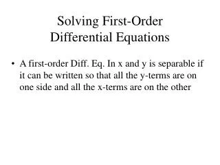
20. 2.4 Separable Equations 2.4.1. Separable equations (page 46-48) Direct If f(x,y) can be expressed as a function of x times a function of y, that is then we say that the differential equation is separable. (5) Example 1

21. Example 2 Solve the initial-value problem Observe that if we use the definite integrals.

22. Example 3 Solve the equation listed in the following The solution can be expressed as (22) B is nonnegative. Thus, (23)

23. Example 4 Free Fall. Suppose that a body of mass m is dropped, from rest, at time t=0. With its displacement x(t) measured down-ward from the point of release, the equation of motion is mx’’ = mg (25a) (25b&c) Let us multiply Eq. (25a) by dx and integrate on x

24. Example 5 Verhulst Population Model.

25. Example 6 Example 7 Sol:

26. Indirect (a) Homogeneous of degree zero Hence

27. Example 8

28. (b) Almost-homogeneous equation can be reduced to homogeneous form by the change of variables x=u+h, y=v+k, where h and k are suitably chosen constants, provided that a1b2-a2b1≠0. Steps for changing the Almost-homogeneous Eq. to homogeneous Eq.

29. 1. Find the intersection (α ,β) 2. 3. 4. It turns to be a homogeneous of degree zero.

30. Example 10 Sol: ; so

31. P.S.

33. Example 11

34. (c) Example 12

36. (c) Isobaric Eqs. Example 13

38. 2.5 Exact equations and integrating factors 2.5.1 Exact differential equations Considering a function F(x,y)=C, the derivative of the function is dF(x,y)=o Considering and

39. Therefore, if (10) Then Mdx+Ndy is an exact differential equation, and according to the definitions Example 1

40. 2.5.2 Integrating factors Even if M and N fail to satisfy Eq. (10), so that the equation is not exact, it may be possible to find a multiplicative factor s(x,y) so that is exact, then we call it an integrating factor, and it satisfied

41. How to find s(x,y) (23) Perhaps an integrating factor s can be found that is a function of x alone. That is sy=0. Then Eq. (23) can be reduced to the differential equation (24) (25) (26)

42. If (My-Nx)/N is not a function of x alone, then an integrating factor s(x) does not exist, but we can try to find s as a function of y alone: s(y). The Eq. (23) reduces to (27) (28)

44. Example 1 Example 1’

45. Example 2

46. Using part known integrating factor to determine the integrating factor of the Eq. Example 3

47. Example 4

48. 2.5.3 Integrating factor of a homogeneous differential Eq. For the homogeneous differential equation M(x,y)dx+N(x,y)dy=0 with the same degree of M and N, if Example 6

49. Example 1 Example 1’

50. Example 2