Basic Probability Distributions: Discrete and Continuous Variables
Dive into Chapter 5 to grasp concepts of random variables, discrete and continuous distributions, binomial and Poisson distributions, and characteristics of normal distribution. Explore numerical properties and examples.

Basic Probability Distributions: Discrete and Continuous Variables
E N D
Presentation Transcript
Chapter 5Basic Probability Distributions :: SunuWibirama :: http://te.ugm.ac.id/~wibirama/notes/
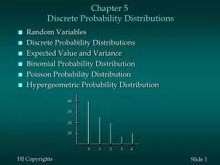
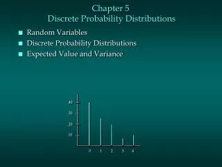
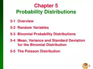
CONTENTS • 5.1. Random variables • 5.2. The probability distribution for a discrete random variable • 5.3. Numerical characteristics of a discrete random variable • 5.4. The binomial probability distribution • 5.5. The Poisson distribution • 5.6 Continuous random variables: distribution function and density function • 5.7 Numerical characteristics of a continuous random variable • 5.8. The normal distribution
Ch. 2 & 3 Ch. 5 Ch. 4 Ch. 2-4 : we used observed sample (what did actually happen) Ch. 5 : combine ch.2-4 by presenting possible outcome along with the relative frequency we expect
5.1 Random Variables Table 5.0. Definition 5.1 • A random variable is a variable that assumes numerical values associated with events of an experiment. • Example: x = number of girls among 14 babies. x is random variable because its values depend on chances
Classification of random variables: discrete continuous
Definition 5.2 • A discrete random variable is one that can assume only a countable number of values. • A continuous random variable can assume any value in one or more intervals on a line.
5.2 The probability distribution for a discrete random variable Definition 5.3 • The probability distribution for a discrete random variable x is a table, graph, or formula that gives the probability of observing each value of x. We shall denote the probability of x by the symbol p(x).
Example A balanced coin is tossed twice and the number x of heads is observed. Find the probability distribution for x.
Solution • Let Hk and Tk denote the observation of a head and a tail, respectively, on the k-th toss, for k = 1, 2. The four simple events and the associated values of x are shown in Table 5.1.
Probability distribution for x • P(x = 0) = p(0) = P(E4) = 0.25. • P(x = 1) = p(1) = P(E2) + P(E3) = 0.25 + 0.25 = 0.5 • P(x = 2) = p(2) = P(E1) = 0.25 Probability distribution for x, the number of heads in two tosses of a coin
Properties of the probability distribution for a discrete random variable x Table 5.2.
5.3 Numerical characteristics of a discrete random variable • Mean or expected value • Variance and standard deviation
5.3.1 Mean or expected value Definition 5.4 • Let x be a discrete random variable with probability distribution p(x). Then the mean or expected value of x is : Definition 5.5 • Let x be a discrete random variable with probability distribution p(x) and let g(x) be a function of x . Then the mean or expected value of g(x) is :
Example 5.6 • Refer to the two-coin tossing experiment and the probability distribution for the random variable x Demonstrate that the formula for E(x) gives the mean of the probability distribution for the discrete random variable x. Solution : If we were to repeat the two-coin tossing experiment a large number of times – say 400,000 times, we would expect to observe x = 0 heads approximately 100,000 times, x = 1 head approximately 200,000 times and x = 2 heads approximately 100,000 times. Calculating the mean of these 400,000 values of x, we obtain
Example cont’d Calculating the mean of these 400,000 values of x, we obtain Thus, the mean of x is 1
5.3.2 Variance and standard deviation Definition 5.6 • Let x be a discrete random variable with probability distribution p(x). Then the variance of x is • The standard deviation of x is the positive square root of the variance of x:
Example5.7 • Refer to the two-coin tossing experiment and the probability distribution for x. Find the variance and standard deviation of x.
Solution • In Example 5.6 we found the mean of x is 1. Then and
5.4 The binomial probability distribution • Example5.8 Suppose that 80% of the jobs submitted to a data-processing center are of a statistical nature. Then selecting a random sample of 10 submitted jobs would be analogous to tossing an unbalanced coin 10 times, with the probability of observing a head (drawing a statistical job) on a single trial equal to 0.80. • Example5.9 Test for impurities commonly found in drinking water from private wells showed that 30% of all wells in a particular country have impurity A. If 20 wells are selected at random then it would be analogous to tossing an unbalanced coin 20 times, with the probability of observing a head (selecting a well with impurity A) on a single trial equal to 0.30.
Model (or characteristics) of a binomial random variable • The experiment consists of n identical trials • There are only 2 possible outcomes on each trial. We will denote one outcome by S (for Success) and the other by F (for Failure). • The probability of S remains the same from trial to trial. This probability will be denoted by p, and the probability of F will be denoted by q ( q = 1-p). • The trials are independent. • The binomial random variable x is the number of S’ in n trials.
The probability distribution, mean and variance for a binomial random variable: The probability distribution: (x = 0, 1, 2, ..., n), where p = probability of a success on a single trial, q=1-p n = number of trials, x= number of successes in n trials =combination of x from n. The mean: The variance:
5.5 The Poisson distribution Characteristics defining a Poisson random variable • The experiment consists of counting the number x of times a particular event occurs during a given unit of time • The probability that an event occurs in a given unit of time is the same for all units. • The number of events that occur in one unit of time is independent of the number that occur in other units. • The mean number of events in each unit will be denoted by the Greek letter
The probability distribution, mean and variance for a Poisson random variable x: • The probability distribution: • Where : = mean of events during the given time periode • The mean: • The variance: ( x = 0, 1, 2,...), e = 2.71828...(the base of natural logarithm).
5.6 Continuous random variables: distribution function and density function • The distinction between discrete random variables and continuous random variables is usually based on the difference in their cumulative distribution functions.
Definition 5.7 • Let be a continuous random variable assuming any value in the interval (- ,+ ). Then the cumulative distribution functionF(x) of the variable is defined as follows: • i.e., F(x) is equal to the probability that the variable assumes values , which are less than or equal to x.
The cumulative area under the curve between -∞ and a point x0 is equal to F(x0).
5.7 Numerical characteristics of a continuous random variable • Definition 5.8
Normal Distribution • The most well known distribution for Discrete Random Variable is Binomial Distribution • The most well known distribution for Continous Random Variable is Normal Distribution • We say x that has a normal distribution if its values fall into a smooth (continuous) curve with a bell-shaped, symmetric pattern, meaning it looks the same on each side when cut down the middle. The total area under the curve is 1.
5.8 Standard Normal Distribution • General density function: • For standardized normal distribution:
Standard Normal Distribution • It’s also called z-distribution • It has a mean of 0 and standard deviation of 1 • Transforming normal random variable x to standard normal random variable z
Homework 1: • Chapter 5, Exercise 5.10, number 1 (page 16)
How to do Homework 2: 1. Get the copy of z-table and use it to compute the result.2. Draw the distribution of fish-length and shade representative areas as stated in problems 1, 2, and 3.3. Use “Finding x from z” to solve problem 1, 2, and 3.
Download All You Need Here: http://te.ugm.ac.id/~wibirama/notes/