Chapter 5 Discrete Probability Distributions
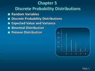
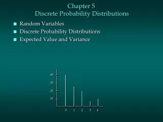
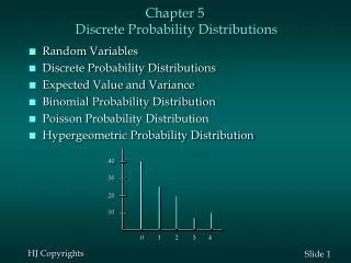
Chapter 5 Discrete Probability Distributions. Random Variables Discrete Probability Distributions Expected Value and Variance Binomial Probability Distribution Poisson Probability Distribution Hypergeometric Probability Distribution. .40. .30. .20. .10.

Chapter 5 Discrete Probability Distributions
E N D
Presentation Transcript
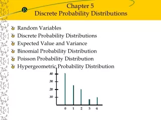
Chapter 5 Discrete Probability Distributions • Random Variables • Discrete Probability Distributions • Expected Value and Variance • Binomial Probability Distribution • Poisson Probability Distribution • Hypergeometric Probability Distribution .40 .30 .20 .10 0 1 2 3 4
Introduction to Probability Distributions • Random Variable • Represents a possible numerical value from a random experiment Random Variables Ch. 5 Ch. 6 Discrete Random Variable Continuous Random Variable
Random Variables • A random variable (随机变量) is a numerical description of the outcome of an experiment.
Random Variables • A discrete random variable(离散随机变量)may assume either a finite number of values or an infinite sequence of values. • A continuous random variable(连续随机变量)may assume any numerical value in an interval or collection of intervals.
Discrete Probability Distributions (离散概率分布) • The probability distribution(概率分布)for a random variable describes how probabilities are distributed over the values of the random variable. • The probability distribution is defined by a probability function(概率函数), denoted by f(x), which provides the probability for each value of the random variable. • The required conditions for a discrete probability function are: f(x) > 0 f(x) = 1 • We can describe a discrete probability distribution with a table, graph, or equation.
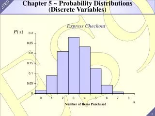
Example: JSL Appliances • Using past data on TV sales (below left), a tabular representation of the probability distribution for TV sales (below right) was developed. Number Units Soldof Daysxf(x) 0 80 0 .40 1 50 1 .25 2 40 2 .20 3 10 3 .05 4 20 4 .10 200 1.00
Example: JSL Appliances • Graphical Representation of the Probability Distribution .50 .40 Probability .30 .20 .10 0 1 2 3 4 Values of Random Variable x (TV sales)
Discrete Uniform Probability Distribution (离散均匀概率函数) • The discrete uniform probability distribution is the simplest example of a discrete probability distribution given by a formula. • The discrete uniform probability function is f(x) = 1/n where: n = the number of values the random variable may assume • Note that the values of the random variable are equally likely.
Expected Value and Variance • The expected value(数学期望), or mean, of a random variable is a measure of its central location. E(x) = = xf(x) • The variance(方差) summarizes the variability in the values of a random variable. Var(x) = 2 = (x - )2f(x) • The standard deviation, , is defined as the positive square root of the variance.
Example: JSL Appliances • Expected Value of a Discrete Random Variable xf(x)xf(x) 0 .40 .00 1 .25 .25 2 .20 .40 3 .05 .15 4 .10 .40 E(x) = 1.20 The expected number of TV sets sold in a day is 1.2
Example: JSL Appliances • Variance and Standard Deviation of a Discrete Random Variable x x - (x - )2 f(x) (x - )2f(x) 0 -1.2 1.44 .40 .576 1 -0.2 0.04 .25 .010 2 0.8 0.64 .20 .128 3 1.8 3.24 .05 .162 4 2.8 7.84 .10 .784 1.660 = The variance of daily sales is 1.66 TV sets squared. The standard deviation of sales is 1.2884 TV sets.
Binomial Probability Distribution(二项分布) • Properties of a Binomial Experiment • The experiment consists of a sequence of n identical trials. • Two outcomes, success and failure, are possible on each trial. • The probability of a success, denoted by p, does not change from trial to trial. • The trials are independent. Stationarity Assumption
Binomial Probability Distribution • Our interest is in the number of successes occurring in the n trials. • We let x denote the number of successes occurring in the n trials.
Binomial Probability Distribution • Number of Experimental Outcomes Providing Exactly x Successes in n Trials where: n! = n(n – 1)(n – 2) . . . (2)(1) 0! = 1
Binomial Probability Distribution • Probability of a Particular Sequence of Trial Outcomes with x Successes in n Trials
Binomial Probability Distribution • Binomial Probability Function where: f(x) = the probability of x successes in n trials n = the number of trials p = the probability of success on any one trial
Example: Evans Electronics • Binomial Probability Distribution Evans is concerned about a low retention rate for employees. On the basis of past experience, management has seen a turnover of 10% of the hourly employees annually. Thus, for any hourly employees chosen at random, management estimates a probability of 0.1 that the person will not be with the company next year. Choosing 3 hourly employees at random, what is the probability that 1 of them will leave the company this year?
Example: Evans Electronics • Using the Binomial Probability Function Let: p = .10, n = 3, x = 1 = (3)(0.1)(0.81) = .243
Example: Evans Electronics • Using the Tables of Binomial Probabilities
2nd Worker 3rd Worker x Probab. 1st Worker L (.1) .0010 3 Leaves (.1) 2 .0090 S (.9) Leaves (.1) L (.1) .0090 2 Stays (.9) 1 .0810 S (.9) L (.1) 2 .0090 Leaves (.1) 1 .0810 S (.9) L (.1) Stays (.9) 1 .0810 Stays (.9) 0 .7290 S (.9) Example: Evans Electronics • Using a Tree Diagram
Binomial Probability Distribution • Expected Value E(x) = = np • Variance Var(x) = 2 = np(1 - p) • Standard Deviation
Example: Evans Electronics • Binomial Probability Distribution • Expected Value E(x) = = 3(.1) = .3 employees out of 3 • Variance Var(x) = 2 = 3(.1)(.9) = .27 • Standard Deviation
Poisson Probability Distribution(泊松概率分布) • A discrete random variable following this distribution is often useful in estimating the number of occurrences over a specified interval of time or space. • It is a discrete random variable that may assume an infinite sequence of values (x = 0, 1, 2, . . . ). • Examples: • the number of knotholes in 14 linear feet of pine board • the number of vehicles arriving at a toll booth in one hour
Poisson Probability Distribution • Properties of a Poisson Experiment • The probability of an occurrence is the same for any two intervals of equal length. • The occurrence or nonoccurrence in any interval is independent of the occurrence or nonoccurrence in any other interval.
Poisson Probability Distribution • Poisson Probability Function where: f(x) = probability of x occurrences in an interval = mean number of occurrences in an interval e = 2.71828
Example: Mercy Hospital • Using the Poisson Probability Function Patients arrive at the emergency room of Mercy Hospital at the average rate of 6 per hour on weekend evenings. What is the probability of 4 arrivals in 30 minutes on a weekend evening? = 6/hour = 3/half-hour, x = 4
Example: Mercy Hospital • Using the Tables of Poisson Probabilities
Hypergeometric Probability Distribution(超几何概率分布) • The hypergeometric distribution is closely related to the binomial distribution. • The key differences are: • the trials are not independent • probability of success changes from trial to trial
Hypergeometric Probability Distribution • Hypergeometric Probability Function for 0 <x<r where: f(x) = probability of x successes in n trials n = number of trials N = number of elements in the population r = number of elements in the population labeled success
Hypergeometric Probability Distribution • Hypergeometric Probability Function • is the number of ways a sample of size n can be selected from a population of size N. • is the number of ways x successes can be selected from a total of r successes in the population. • is the number of ways n – x failures can be selected from a total of N – r failures in the population.
例:在一个口袋中装有30个球,其中有10个红球,其余为白球,这些球除颜色外完全相同.游戏者一次从中摸出5个球.摸到4个红球就中一等奖,那么获一等奖的概率是多少? • 解:由题意可见此问题归结为超几何分布模型。 • 其中N = 30. r = 10. n = 5. • P(一等奖) = P(X=4 or 5) = P(X=4) + P(X=5) • P(X=4) = C(4,10)*C(1,20)/C(5,30) • P(X=5) = C(5,10)*C(0,20)/C(5,30) • P(一等奖) = 106/3393
Example: Neveready • Hypergeometric Probability Distribution Bob Neveready has removed two dead batteries from a flashlight and inadvertently mingled them with the two good batteries he intended as replacements. The four batteries look identical. Bob now randomly selects two of the four batteries. What is the probability he selects the two good batteries?
Example: Neveready • Hypergeometric Probability Distribution where: x = 2 = number of good batteries selected n = 2 = number of batteries selected N = 4 = number of batteries in total r = 2 = number of good batteries in total