Download
1 / 36
370 likes | 614 Views
ECOSMO an ECOSystem Model coupled physics-lower trophic level dynamics. General Overview. Basic equations Towards model equations: vertical integration Model equations and approximations Air-sea and air-ice-ocean fluxes Lower trophic level dynamics Numerical schemes

E N D
ECOSMO an ECOSystem Model coupled physics-lower trophic level dynamics
General Overview • Basic equations • Towards model equations: vertical integration • Model equations and approximations • Air-sea and air-ice-ocean fluxes • Lower trophic level dynamics • Numerical schemes • Grid- and slab information • Model flow, main program • Literature • Additional features • New set-up Irina
Basic equations • Reynolds equations, hydrostatic approximation, conservation equation: mass (volume), salt mass, heat and tracer mass (nutrients, biomass etc…) • Vertical integration and boundary conditions results in model equations
Transport model equations : subroutines motmit, druxav, konv
Model equations for T and S(and other tracers) subroutine strom3
More model equations subroutine konti subroutine sor, sorcof subroutine estate
Turbulence closure • Stationarity • local production and local dissipation of turbulent kinetic energy balance, • advection and diffusion of turbulent kinetic energy can be neglected
Vertical integration for one model layer k from zk-zk-1:Horizontal transport
Turbulence closure subroutine druxav
Dynamic sea ice model: subroutine icemod, icevel • 3 state variables: • -Ice compactness Ai, • -level ice thickness hi • - ridging ice thickness hr • continuum approach, conservation equations for open water area, level ice thickness, ridging ice thickness • Hibler type ice dynamics: viscous-plastic, elliptical yield curve, normal flow rule
Conservation equation for ice stages: compactness (open water and thin ice), level ice, ridged ice
Mechanic deformation functions 3 cases: • Ai<1 and convergent or divergent flow field, or divergent flow field ice transport change only ice concentration • Ai=1, ice thickness below critical value (0.1m), convergent flow field ice transport results in rafting: level ice thickness change • Ai=1, ice thickness above critical value, convergent flow field ice transport results in ridging: level ice thickness change
Air sea fluxes : subroutine fluxes • Based on Monin-Obukhov similarity theory: • - MONIN and OBUKHOV, 1954 • - LAUNIAINEN and VIHMA, 1990 • 2m Tair, spec. humidity are up-scaled to 10m-ref heights • Upscaling, cd exchange coefficients and fluxes depend on atmospheric stability
Lower trophic level dynamics: coupling vs. transport equations subroutine strom3 calls subroutine bio
Lower trophic level dynamics: subroutine bio 12 biological and chemical variables: Phytoplankton: Pd - diatoms; Pf - flagellates; Zooplankton: Zs, Z l – micro and macro-zooplankton; Nitrogen: NH4 - ammonium; NO2- nitrite;NO3 - nitrate; Phosphorus: PO4 - phosphate; Silica:SiO2 - silicate; SiO2•2H2O- biogenic opal; O2–Oxygen, D - detritus
Biological state variables parameter (nbio=14) dimension Tc(ndrei,nbio) ibio=1,nbio ibio = 1,2 reserved for T,S ibio = 3,nbio: 3 4 Phytoplankton: Ps – flagellates; Pl- diatoms; 5 6 Zooplankton: Zs, Z l – micro and macro-zooplankton; 7 D - detritus; 8 9 10 Nitrogen: NH4 - ammonium; NO2- nitrite;NO3 - nitrate; 11 Phosphorus: PO4 - phosphate; 12 14 Silica:SiO2 - silicate; SiO2•2H2O- biogenic opal; 13 O2–Oxygen.
Biological reactions in the model :term RCis Dxbi(ndrei,nbio) Subroutine bio (Tc,dd,dz,sh_wave,sh_depth)
Numerics: basic information • Semi-implicit: -implicit: barotropic pressure gradients, turbulent vertical exchange -explicit: convective terms, baroclinic pressure gradients, horizontal turbulent diffusion • Convective or nonlinear terms: energy and enstrophy conserving scheme Arakawa J7 • Rotation of corriolis term (C-grid) • Upstream advection scheme (2d) for T,S and bio-parameter • Free surface and bottom depth resolving coordinates application of kinematic boundary conditions necessary
Model grid: Arakawa C-grid horizontal Columns n (j) NW=(1,1) Rows m (i) • TC(i,j) X U(i,j) • TC(i,j+1) X U(i,j+1) +V(i,j) +V(i,j+1) • TC(i+1,j) X U(i+1,j) • TC(i+1,j+1) X U(i+1,j+1) +V(i+1,j+1) +V(i+1,j)
Model grid: vertical grid Surface layer: 1 +w (k) Av(k) ilo (k) • Av and w are not defined at the lower boundary of the bottom layer • Av(1)=0, i.e. at the sea surface • w(1) is the first guess for solving the equation system for the sea surface elevation • TC(k) +w (k+1) Av(k+1) • TC(k+1)
Organisation of slabs: Counting wet grid points c----------------------------------------------------------------------- c set grid index arrays c----------------------------------------------------------------------- lwe = 0 nwet=0 do k=1,n lwa = lwe+1 lwe = indend(k) do lw=lwa,lwe i = iwet(lw) lump = lazc(lw) jjc(i,k) = 1 iindex(i,k) = nwet id3sur(lw) = nwet+1 do jj=1,lump nwet = nwet+1 enddo izet(i,k) = lw enddo enddo • Start with NW grid point, at the sea surface • 2-d arrays: outer loop columns, inner loop rows • 3-d arrays: outer loop, columns, than rows, inner loop depth layers
Relevant arrays and dimensions • compressed 3-d arrays of dimension ndrei UC(ndrei) • compressed 2-d arrays of dimension khor zac(khor) • iindex(i,j) help array to address wet grid from i,j,k arrays i,j,k known respective uc=uc(iindex(i,j)+k) • jjc(i,k) mask array, =1 if wet, =0 if land point • lazc(khor): number of layers for compressed 2-d arrays • iwet (khor): i-index(row) for compressed 2-d arrays • indend(k): end index of compressed arrays for
Literature model description • Backhaus J. O. (1983) A semi-implicit scheme for the shallow water equations for application to shelf sea modelling. Continental Shelf Research, 3,243-254. • Backhaus J. O. (1985) A three-dimensional model for the simulation of shelf sea dynamics. Deutsche Hydrographische Zeitschrifi, 38, 165-187. • Schrum, C. (1997): Thermohaline stratification and instabilities at tidal mixing fronts. Results of an eddy resolving model for the German Bight. Cont. Shelf. Res., 17(6), 689-716. • Schrum, C, Backhaus, J. O. (1999): Sensitivity of atmosphere-ocean heat exchange and heat content in North Sea and Baltic Sea. A comparitive assessment. Tellus 51A. 526-549. • Schrum, C, Alekseeva, I, St. John, M (2006): Development of a coupled physical–biological ecosystem model ECOSMO Part I: Model description and validation for the North Sea, Journal of Marine Systems, doi:10.1016/j.jmarsys.2006.01.005.
Access to model code and literature • ftp://ftp.uib.no/ path: /var/ftp/pub/gfi/corinna/ECOSMO
Additional features (not in basic version) • 3-d wetting and drying, mass conserving • Groundwater runoff module • Particle tracking module (online) • IBM parameterized for larvae fish growing (temperature based and food consumption)
Setting up a new configuration • Attention required: • ngro array size to be set in C_model.f, it needs to be ngro=max((m*(ilo*20+10),(kasor*8)), for current configuration set to m*(ilo*20+10) • consider exclusion of boundary points for iteration in kotief! currently weak programming • 3 frame lines are necessary in the west and north, only 2 frame lines in the south and east • consider 3 equal boundary lines at the open boundaries