Download
1 / 15
160 likes | 348 Views
CE 394K.2 Hydrology, Lecture 2 Hydrologic Systems. Hydrologic systems and hydrologic models How to apply physical laws to fluid systems Intrinsic and extrinsic properties of fluids Reynolds Transport Theorem Continuity equation

E N D
CE 394K.2 Hydrology, Lecture 2Hydrologic Systems • Hydrologic systems and hydrologic models • How to apply physical laws to fluid systems • Intrinsic and extrinsic properties of fluids • Reynolds Transport Theorem • Continuity equation • Reading – Applied Hydrology, Sections 1.2 to 1.5 and 2.1 to 2.3
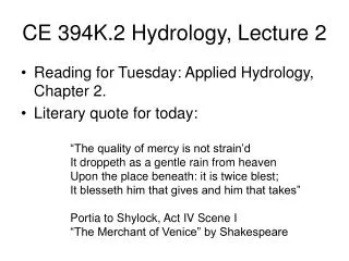
Hydrologic System Take a watershed and extrude it vertically into the atmosphere and subsurface, Applied Hydrology, p.7- 8 A hydrologic system is “a structure or volume in space surrounded by a boundary, that accepts water and other inputs, operates on them internally, and produces them as outputs”
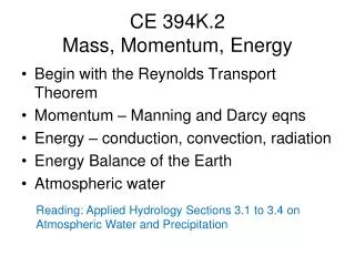
System Transformation Transformation Equation Q(t) = I(t) Outputs, Q(t) Inputs, I(t) A hydrologic system transforms inputs to outputs Hydrologic Processes I(t), Q(t) Hydrologic conditions I(t) (Precip) Physical environment Q(t) (Streamflow)
Stochastic transformation System transformation f(randomness, space, time) Outputs, Q(t) Inputs, I(t) Hydrologic Processes I(t), Q(t) How do we characterize uncertain inputs, outputs and system transformations? Hydrologic conditions Physical environment Ref: Figure 1.4.1 Applied Hydrology
Views of Motion • Eulerian view (for fluids – e is next to f in the alphabet!) • Lagrangian view (for solids) Fluid flows through a control volume Follow the motion of a solid body
Reynolds Transport Theorem • A method for applying physical laws to fluid systems flowing through a control volume • B = Extensive property (quantity depends on amount of mass) • b = Intensive property (B per unit mass) Rate of change of B stored within the Control Volume Total rate of change of B in fluid system (single phase) Outflow of B across the Control Surface
Reynolds Transport Theorem Rate of change of B stored in the control volume Total rate of change of B in the fluid system Net outflow of B across the control surface
Continuity Equation B = m; b = dB/dm = dm/dm = 1; dB/dt = 0 (conservation of mass) r = constant for water or hence
Continuity equation for a watershed Hydrologic systems are nearly always open systems, which means that it is difficult to do material balances on them I(t) (Precip) What time period do we choose to do material balances for? dS/dt = I(t) – Q(t) Q(t) (Streamflow) Closed system if
Continuous and Discrete time data Figure 2.3.1, p. 28 Applied Hydrology Continuous time representation Sampled or Instantaneous data (streamflow) truthful for rate, volume is interpolated Can we close a discrete-time water balance? Pulse or Interval data (precipitation) truthful for depth, rate is interpolated