Chapter 12 Judgment and Choice

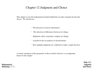
1. Chapter 12 Judgment and Choice • This chapter covers the mathematical models behind the way that consumer decide and choose. We will discuss • The detection of sensory information • The detection of differences between two things • Judgments where consumers compare two things • A model for the recognition of advertisements • How multiple judgments are combined to make a single decision As usual, estimation of the parameters in these models will serve as an important theme for this chapter

2. There Are Two Different Types of Judgments • Absolute Judgment • Do I see anything? • How much do I like that? • Comparative Judgment • Does this bagel taste better than that one? • Do I like Country Time Lemonade better than Minute Maid? Psychologists began investigating how people answer these sorts of questions in the 19th Century

3. The Early Concept of a “Threshold” Absolute Detection 1.0 Pr(Detect) .5 0 n Physical measurement Difference Detection 1.0 Pr(n Perceived > n2) .5 0 n1 n2 n3

4. But the Data Never Looked Like That 1.0 .5 Pr(Detect) 0 n

5. A Simple Model for Detection si is the psychological impact of stimulus i If si exceeds the threshold, you see/hear/feel it Pr[Detect stimulus i] = Pr[si s0] . We make this assumption ei ~ N(0, 2) so that which then implies We also assume

6. Our Assumptions Imply That the Probability of Detection Is… (Note missing left bracket in Equation 12.6 in book.) Converting to a z-score we get (Note missing subscript i on the z in book)

7. Making the Equation Simpler But since the normal distribution is symmetric about 0 we can say:

8. Graphical Picture of What We Just Did 0 Pr(Detection) 0

9. A General Rule for Pr(a > 0)Where a Is Normally Distributed For a ~ N[E(a), V(a)] we have Pr [a  0] =  [E(a) /  V(a)]

10. So Why Do Detection Probabilities Not Look Like a Step Function?

11. Paired Comparison Data: Pr(Row Brand > Column Brand)

12. Draw sj Draw si Is si > sj? Assumptions of the Thurstone Model ei ~ N(0, ) Cov(ei, ej) = ij = rij

13. Deriving the E(si - sj) and V (si - sj) pij = Pr(si > sj ) = Pr(si -sj > 0)

14. Predicting Choice Probabilities For a ~ N[E(a), V(a)] we have Pr [a  0] =  [E(a) /  V(a)] Below si - sj plays the role of "a"

15. Thurstone Case III = 0 = 1 How many unknowns are there? How many data points are there?

16. Unweighted Least Squares Estimation

17. Conditions Needed for Minimizing f

18. Minimum Pearson 2 Same model: Different objective function

19. Matrix Setup for Minimum Pearson 2 V(p) = V

20. Modified Minimum Pearson 2 Minimum Pearson 2 Simplifies the derivatives, and reduces the computational time required

21. Definitions and Background for ML Estimation Assume that we have two possible events A and B. The probability of A is Pr(A), and the probability of B is Pr(B). What are the odds of two A's on two independent trials? Pr(A) • Pr(A) = Pr(A)2 In general the Probability of p A's and q B's would be Note these definitions and identities: fij = npij

22. ML Estimation of the Thurstone Model According to the Model According to the general alternative

23. Categorical or Absolute Judgment Love Like Dislike Hate [ ] [ ] [ ] [ ] s1 s2 s3 1 2 3 4 Love Like Dislike Hate Brand 1 Brand 2 Brand 3 .20 .30 .20 .30 .10 .10 .60 .20 .05 .10 .15 .70

24. Cumulated Category Probabilities Love Like Dislike Hate Brand 1 Brand 2 Brand 3 .20 .30 .20 .30 .10 .10 .60 .20 .05 .10 .15 .70 Raw Probabilities Brand 1 .20 .50 .70 1.00 Cumulated Probabilities Brand 2 .10 .20 .80 1.00 Brand 3 .05 .15 .30 1.00

25. The Thresholds or Cutoffs c0 = - c4 = + c1 c2 c3 (cJ-1)

26. A Model for Categorical Data ei ~ N(0, 2) Probability that the discriminal response to item i is less than the upper boundary for category j Probability that item i is placed in category j or less

27. The Probability of Using a Specific Category (or Less) Pr [a  0] =  [E(a) /  V(a)] Below ci - sj is plays the role of "a"

28. The Theory of Signal Detectability