Temporal Planning
Temporal Planning. Planning with Temporal and Concurrent Actions. Literature. Malik Ghallab, Dana Nau, and Paolo Traverso. Automated Planning – Theory and Practice , chapter 13-14. Elsevier/Morgan Kaufmann, 2004. Why Explicit Time?. assumption A6: implicit time

Temporal Planning
E N D
Presentation Transcript
Temporal Planning Planning with Temporal and Concurrent Actions
Literature • Malik Ghallab, Dana Nau, and Paolo Traverso. Automated Planning – Theory and Practice, chapter 13-14. Elsevier/Morgan Kaufmann, 2004. Temporal Planning
Why Explicit Time? • assumption A6: implicit time • actions and events have no duration • state transitions are instantaneous • in reality: • actions and events do occur over a time span • preconditions not only at beginning • effects during or even after the action • actions may need to maintain partial states • events expected to occur in future time periods • goals must be achieved within time bound Temporal Planning
Overview • Actions and Time Points • Interval Algebra and Quantitative Time • Planning with Temporal Operators Temporal Planning
Time • mathematical structure: • set with transitive, asymmetric ordering operation • discrete, dense, or continuous • bounded or unbounded • totally ordered or branching • temporal references: • time points (represented by real numbers) • time intervals (pair of real numbers) • temporal relations: • examples: before, during Temporal Planning
Causal vs. Temporal Analysis of Actions • example: load(crane2, cont5, robot1, interval6) • causal analysis (what propositions hold?): • what propositions will change (effects) • what propositions are required (preconditions) • temporal analysis (when propositions hold?): • when other, related assertions can/cannot be true • reason over: • time periods during which propositions must hold • time points at which values of state variables change Temporal Planning
Temporal Databases • maintain temporal references for every domain proposition • when does it hold • when does it change value • functionality: • assert new temporal relations • querying whether temporal relation holds • check for consistency • planner attempts to assert relations among temporal references Temporal Planning
Temporal References Example: Container Loading • load container c onto robot r at location l • t1: instant at which robot r enters location l • t2: instant at which robot r stops at location l • i1=[t1,t2]: interval corresponding to r entering l • t3: instant at which the crane starts picking up c • t4: instant at which crane finishes putting c on r • i2=[t3,t4]: interval corresponding to picking up and loading c • t5: instant at which c begins to be loaded onto r • t6: instant at which c is no longer loaded onto r • i3=[t5,t6]: interval corresponding to c being loaded onto r Temporal Planning
Temporal Relations Example: Container Loading • assumption: crane is allowed to pick up container as soon as robot has entered location • possible temporal sequences: • t1 < t3 < t2 < t4 = t5 < t6 (see figure) or • t1 = t3 or t2 = t3 or t2 < t3 entering t1 t2 loaded t5 t6 picking up and loading t3 t4 Temporal Planning
Example: Temporal Relations as Constraint Networks < t1 t2 < t5 < t6 ≤ = < t3 t4 before i1 i3 starts before meets i2 Temporal Planning
Point Algebra (PA): Relations and Constraints • possible primitive relations P between instants t1 and t2: P = {<,=,>} • t1 before t2: [t1<t2] • t1 equal to t2: [t1=t2] • t1 after t2: [t1>t2] • possible qualitative constraints R between instants: • sets of the above relations (interpret as disjunction) • R = 2P = {∅, {<}, {=}, {>}, {<,=}, {<,>}, {=,>}, P} Temporal Planning
Container Loading Example: PA Constraints • [t1 {<} t2] • [t1 {<,=} t3] • [t2 {<} t5] • [t3 {<} t4] • [t4 {=} t5] • [t5 {=} t4] • [t5 {<} t6] {<} t1 t2 {<} t5 {<} t6 {<,=} {=} {<} t3 t4 Temporal Planning
PA: Combining Constraints • usual set operations: • ∩, ∪ etc. • composition (noted ∙): • let r, q∈R • if [t1rt2] and [t2qt3] • then [t1r∙qt3] • r∙q as defined in composition table PA composition table Temporal Planning
distributive (r ∪ q) ∙s = (r ∙ s) ∪ (q ∙ s) s∙ (r ∪ q) = (s ∙ r) ∪ (s ∙ q) symmetrical constraint r’ of r: [t1rt2] iff [t2r’t1] obtained by replacing in r: < with > and vice versa (r ∙ q)’ = q’ ∙ r’ (R,∪,∙) is an algebra: R is closed under ∪ and ∙ ∪ is an associative and commutative operation identity element for ∪ is ∅ is an associative operation identity element for ∙ is {=} PA: Properties of Combined Constraints Temporal Planning
PA: Constraint Propagation • given constraints: • [t1rt2] • [t1qt3] • [t3st2] • implied constraint: • [t1r ∩ q∙st2] • inconsistency: • if r ∩ q∙s= ∅ q∙s r t1 t2 q s t3 Temporal Planning
Container Loading Example: Constraint Propagation • path: t4-t5-t6: [t4=t5] ∙ [t5<t6] implies [t4<t6] • path: t2-t1-t3: [t2>t1] ∙ [t1≤t6] implies [t2Pt3] • path: t2-t5-t4: [t2<t5] ∙ [t5=t4] implies [t2<t4] • path: t2-t3-t4: [t2Pt3] ∙ [t3<t4] implies [t2Pt4] {<} t1 t2 {<} t5 {<} t6 {<} {<,=} {P} {=} {<} {P} {<} t3 t4 [t2<t4] Temporal Planning
PA Constraint Networks • A binary PA constraint network is a directed graph (X,C), where: • X = {t1,…,tn} is a set of instant variables (nodes), and • C⊆ X×X (the edges), cij is labelled by a constraint rij∈R iff [ti rij tj] holds. • A tuple 〈v1,…,vk〉 of real numbers is a solution for (X,C) iff ti=vi satisfy all the constraints in C. • (X,C) is consistent iff there exists at least one solution. Temporal Planning
Primitives in Consistent Networks • Proposition: A PA network (X,C) is consistent iff • there is a set of primitives pij∈ rij for every cij∈C such that • for every k: pij∈(pik ∙pkj) • note: not interested in solution, just consistency (qualitative solution) Temporal Planning
Redundant Networks • A primitive pij ∈ rij is redundant if there is no solution in which [ti pij tj] holds. • idea: filter out redundant primitives until • either: no more redundant primitives can be found • or: we find a constraint that is reduced to ∅ (inconsistency) Temporal Planning
Path Consistency: Pseudo Code pathConsistency(C) while¬C.isStable() do for each k : 1≤k≤ndo for each pair i,j: 1≤i<j≤n,i≠k, j≠kdo cij cij∩ [cik∙ckj] ifcij=∅ then return inconsistent Temporal Planning
Path Consistency: Properties • algorithm pathConsistency(C) is: • incomplete for general CSPs • complete for PA networks • network (X,C) is minimal if it has no redundant primitives in a constraint • algorithm pathConsistency(C) does not guarantee a minimal network Temporal Planning
Overview • Actions and Time Points • Interval Algebra and Quantitative Time • Planning with Temporal Operators Temporal Planning
Extended Example: Inspect and Seal • every container must be inspected and sealed: • inspection: • carried out by the crane • must be performed before or after loading • sealing: • carried out by robot • before or after unloading, not while moving • corresponding intervals: • iload, imove, iunload, iinspect, iseal Temporal Planning
Inspect and Seal Example: Interval Constraint Network imove before iload before before before or after before or after iunload before iinspect before iseal Temporal Planning
Inspect and Seal Example: Qualitative Instant Constraints • Let i be an interval. • i.b and i.e denote two end time points • [i.b≤i.e] constraint: beginning before end • [iload before imove]: • [iload.b≤iload.e] and[imove.b≤imove.e] and • [iload.e<imove.b] • [imove before-or-after iseal]: • [imove.e<iseal.b] or • [iseal.e<imove.b] disjunction cannot be translated into binary PA constraint Temporal Planning
i1 before i2: [i1bi2] i1 meets i2: [i1mi2] i1 overlaps i2: [i1oi2] i1 starts i2: [i1si2] i1 during i2: [i1di2] i1 finishes i2: [i1fi2] i1 i2 i1 i2 i1 i2 i1 i2 i1 i2 i1 i2 Interval Algebra (IA): Relations Temporal Planning
i1 i2 IA: Relations and Constraints • possible primitive relations P between intervals i1 and i2: • just described: [i1bi2], [i1mi2], [i1oi2], [i1si2], [i1di2], [i1fi2] • symmetrical: [i1b’i2], [i1m’i2], [i1o’i2], [i1s’i2], [i1d’i2], [i1f’i2] • i1 equals i2: [i1ei2] • possible qualitative constraints R between instants: • sets of the above relations (interpret as disjunction) • R = 2P = {∅, {b}, {m}, {o},…, {b,m}, {b,o},…, {b,m,o},…, P} • examples: while = {s,d,f}; disjoint = {b,b’} Temporal Planning
Operations on Relations • set operations: ∩, ∪ etc. • composition: ∙ Temporal Planning
i1 i2 i3 i1 i2 i3 i3 Properties of Composition • transitive • if [i1ri2] and [i2qi3] then [i1 (r ∙ q) i3] • distributive • (r ∪ q) ∙s = (r ∙ s) ∪ (q ∙ s) • s∙ (r ∪ q) = (s ∙ r) ∪ (s ∙ q) • not commutative • [i1 (r ∙ q) i2] does not imply [i1 (q ∙ r) i2] • example: d∙b = {b}; b ∙ d = {b,m,o,s,d} [i1 (d ∙ b) i3] [i1 (b ∙ d) i3] Temporal Planning
Inspect and Seal Example: Interval Constraint Propagation imove • iinspect-imove-iunload: [iinspect {b} ∙ {b} iunload] = [iinspect {b} iunload] • iinspect-iload-iseal: [iinspect {b,b’} ∙ {b} iseal] = [iinspectPiseal] {b} iload {b} {b} {b,b’} iunload {b,b’} {b} {b} iinspect {b} P iseal Temporal Planning
IA Constraint Networks • A binary IA constraint network is a directed graph (X,C), where: • X = {i1,…,in} is a set of interval variables ij=(ij.b, ij.e), where ij.b≤ij.e, and • C⊆ X×X (the edges), cij is labelled by a constraint rij∈R iff [ii rij ij] holds. • A tuple 〈v1,…,vk〉 of pairs of real numbers (vi.b, vi.e) is a solution for (X,C) iff vi.b≤vi.eii=vi satisfy all the constraints in C. • (X,C) is consistent iff there exists at least one solution. Temporal Planning
Primitives in Consistent Networks • Proposition: A IA network (X,C) is consistent iff • there is a set of primitives pij∈ rij for every cij∈C such that • for every k: pij∈(pik ∙pkj) • idea: filter out redundant primitives using path consistency algorithm until • either: no more redundant primitives can be found • or: we find a constraint that is reduced to ∅ (inconsistency) • note: path consistency not complete for IA networks Temporal Planning
Example: Quantitative Temporal Relations • ship: Uranus • arrives within 1 or 2 days • will leave either with • light cargo (stay docked 3 to 4 days) or • full load (stay docked at least six days) • ship: Rigel • to be serviced on • express dock (stay docked 2 to 3 days) • normal dock (stay docked 4 to 5 days) • must depart 6 to 7 days from now • Uranus must depart 1 to 2 days after Rigel arrives Temporal Planning
Example: Quantitative Temporal Constraint Network [3,4] or [6,∞] • 5 instants related by quantitative constraints • e.g. (2 ≤ DRigel-ARigel≤ 3) ⋁ (4 ≤ DRigel-ARigel≤ 5) • possible questions: • When should the Rigel arrive? • Can it be serviced on a normal dock? • Can the Uranus take a full load? AUranus DUranus [1,2] [1,2] now ARigel [2,3] or [4,5] [6,7] DRigel Temporal Planning
Overview • Actions and Time Points • Interval Algebra and Quantitative Time • Planning with Temporal Operators Temporal Planning
Temporally Qualified Expressions (tqe) • tqe: expression of the form:p(o1,…,ok)@[tb,te[where: • p is a flexible relation in the planning domain, • o1,…,okare object constants or variables, and • tb,te are temporal variables such that tb<te. • tqep(o1,…,ok)@[tb,te[ asserts that: • for every time point t: tb≤t<te implies that p(o1,…,ok) holds • [tb,te[ is semi-open to avoid inconsistencies Temporal Planning
Temporal Database • A temporal database is a pair Φ=(F,C) where: • F is a finite set of tqes, • C is a finite set of temporal and object constraints, and • C has to be consistent, i.e. there exist possible values for the variables that meet all the constraints. Temporal Planning
robot r1 is at location loc1 robot r2 moves from location loc2 to location loc3 Φ = ({ at(r1,loc1)@[t0,t1[, at(r2,loc2)@[t0,t2[, at(r2,path)@[t2,t3[, at(r2,loc3)@[t3,t4[, free(loc3)@[t0,t5[, free(loc2)@[t6,t7[ }, { adjacent(loc2,loc3), t2<t6<t5<t3 }) free(loc3) at(r1,loc1) at(r2,loc2) at(r2,path) at(r2,loc3) free(loc2) Temporal Database: Example t0 t1 t0 t2 t3 t4 < t5 t0 < < t6 t7 Temporal Planning
Inference over tqes • A set F of tqes supports a (single) tqee=p(v1,…,vk)@[tb,te[ iff: • there is a tqep(o1,…,ok)@[t1,t2[ in F and • there is a substitution σ such that: • σ(p(v1,…,vk)) = p(o1,…,ok). • An enabling condition for e in F is the conjunction of the following constraints: • t1≤tb, te≤t2 and • the variable binding constraints in σ. Temporal Planning
Inference over tqes: Example • F = {at(r1,loc1)@[t0,t1[, at(r2,loc2)@[t0,t2[, at(r2,path)@[t2,t3[, at(r2,loc3)@[t3,t4[, free(loc3)@[t0,t5[, free(loc2)@[t6,t7[ } • F supports free(l)@[t,t’[ • with enabling conditions: • t0≤t, t’≤t5, and l=loc3, or • t6≤t, t’≤t7, and l=loc2. Temporal Planning
Inference over Sets of tqes • A set F of tqes supports a set E of tqes iff: • there is a substitution σ such that: • F supports every tqee∈E using substitution σ. • The set of enabling conditions for a single tqee in F is denoted Θ(e/F). • The set of enabling conditions for a set of tqes E in F is denoted Θ(E/F). Temporal Planning
Inference over Temporal Databases • A temporal database Φ=(F,C) supports a set E of tqes iff: • F supports E and • there is an enabling condition c∈Θ(E/F) that is consistent with C. • A temporal database Φ=(F,C) supports another temporal database Φ’=(F’,C’) iff: • F supports F’ and • there is an enabling condition c∈Θ(F’/F) such that • C’∪c is consistent with C. • A temporal database Φ=(F,C) entails another temporal database Φ’=(F’,C’) iff: • F supports F’ and • there is an enabling condition c∈Θ(F’/F) such that • C entails C’∪c. Temporal Planning
at(r,l) at(r,path) at(r,l’) free(l) free(l’) Temporal Planning Operators: Example • move(r,l,l’)@[tb,te[ • preconditions: at(r,l)@[t1,tb[, free(l’)@[t2,te[ • effects: at(r,path)@[tb,te[, at(r,l’)@[te,t3[, free(l’)@[t4,t5[ • constraints: tb<t4<t2, adjacent(l,l’) move(r,l,l’) t1 tb t3 t2 t4 t5 Temporal Planning
Temporal Planning Operators • A temporal planning operator o is a tuple (name(o), precond(o), effects(o), constr(o)), where: • name(o) is an expression of the form a(x1,…,xk,tb,te) such that: • a is a unique operator symbol, • x1,…,xk are the object variables appearing in o, and • tb,te are temporal variables in o, • precond(o) and effects(o) are sets of tqes, and • constr(o) is a conjunction of the following constraints: • temporal constraints on tb,te and possibly further time points, • rigid relations between objects, and • binding constraints of the form x=y, x≠y, or x∈D. Temporal Planning
Applicability of Temporal Planning Operators • A temporal planning operator o is applicable to a temporal database Φ=(F,C) iff: • precond(o) is supported by F and • there is an enabling condition c in Θ(precond(o)/F) such that: • C∪ constr(o) ∪c is consistent. • The result of applying an applicable action a to Φ is a set of possible temporal databases • γ0(Φ,a) = { (F ∪ effects(a), C∪ constr(a) ∪c) | c∈ Θ(precond(a)/F) } Temporal Planning
at(r1,loc1) at(r2,loc2) at(r2,path) at(r2,loc3) free(loc3) free(loc2) Applicable Operator: Example • operator: move(r,l,l’)@[tb,te[ • at(r1,loc1)@[t0,t1[ supports at(r,l)@[t’1,tb[ • free(loc2)@[t6,t7[ supports free(l’)@[t’2,te[ • enabling condition: {r=rob1, l=loc1, l=loc1, t0≤t’1, tb≤t1, t6≤t’2, te≤t7} • consistent • move(r1,loc1,loc2) is applicable t0 t1 t0 t2 t3 t4 < t5 t0 < < t6 t7 Temporal Planning
Domain Axioms: Example • no object can be in two places at the same time:{at(r,l)@[tb,te[, at(r’,l’)@[t’b,t’e[} → (r≠r’) ⋁ (l=l’) ⋁ (te≤t’b) ⋁ (t’e≤tb) • every location can be occupied by one robot only: {at(r,l)@[t1,t’1[, free(l’)@[t2,t’2[} → (l≠l’) ⋁ (t’1≤t2) ⋁ (t’2≤t1) Temporal Planning
Domain Axioms • A domain axiomα is an expression of the form: cond(α) → disj(α) where: • cond(α) is a set of tqes and • disj(α) is a disjunction of temporal and object constraints. • A temporal database Φ=(F,C) is consistent with α iff: • cond(α) is supported by F and • for every enabling condition c1∈ Θ(cond(α)/F) • there is at least one disjuct c2∈ disj(α) such that • C∪c1∪c2 is consistent. Temporal Planning
Temporal Planning Domains • A temporal planning domain is a triple D = (SΦ,O,X) where: • SΦ is the set of all temporal databases that can be defined with the constraints and the constant, variable, and relation symbols in our representation, • O is the set of temporal planning operators, and • X is a set of domain axioms. Temporal Planning
Temporal Planning Problems • A temporal planning problem in D is a triple P = (D,Φ0,Φg) where: • D = (SΦ,O,X) is a temporal planning domain, • Φ0=(F,C) is a database in SΦ that satisfies the axioms in X. • represents the initial scenario including: • initial state of the world • predicted evolution independent of planned actions • Φg=(G,Cg) is a database in SΦ where: • G is a set of tqes representing the goals of the problem • Cg are object and temporal constraints on variables in G. Temporal Planning