Spatial Statistics in Ecology: Continuous Data
Spatial Statistics in Ecology: Continuous Data. Lecture Three. Recall and Introduction to Continuous Processes. Recall from last time that point patterns can be visualized as continuous data by applying Kernel Estimation


Spatial Statistics in Ecology: Continuous Data
E N D
Presentation Transcript
Spatial Statistics in Ecology: Continuous Data Lecture Three
Recall and Introduction to Continuous Processes • Recall from last time that point patterns can be visualized as continuous data by applying Kernel Estimation • Much of the data we use in ecology is not localized at x,y but is instead local samples of a process that takes place over a large area with intensity varying depending on the location of the sample
This type of data is called CONTINOUS • Can you think of the type of data ecologists collect that is continuous? • Some obvious examples we have already mentioned are rainfall or temperature.
How are they different? • Continuous process are very different than point patterns • In point pattern analysis we look at locations of “events” • With continuous data we try to understand the spatial distribution of values of an attribute over a large study region
Objective • The objective in studying continuous processes is is to model the pattern of variability and to establish factors to which this pattern relates • Imagine a rainfall map which showed a line of higher values along the vertical axis. What might this tell you about the process this pattern relates to? If you are thinking of a mountain range your on the right track! • We can use these models to PREDICT the values of attributes at points that have not been sampled.
Bandwidth is all important • This raises an obvious issue with modelling continuous processes…..the scale (in this case the bandwidth) must be carefully considered. • Striking a balance between too small a bandwidth (and thus possible very high errors for some predictions) and a large bandwidth (low errors in all predictions) is essential. • Knowledge of the biology and ecology of the system is important to making these types of judgments.
Visualizing Continuous Processes Proportional symbol map The simplest method would be to create a surface using the mean values of the process over space. What problems can you see with this method? The color represents variation in intensity of variable A The area is proportional to the data value of variable B
Exploring continuous processes To explore continuous processes we create a surface of means to assess locations where we do not have observations using a method called a WEIGHTED AVERAGE Points closer to the event will have higher weights than point further away
Kernel Estimation Point Pattern Similar to creating a TREND SURFACE for point patterns, kernel estimation is the most common method to explore the trends for continuous processes Continuous process Can anyone tell what the difference is?
Kernel – first-order effect • Point patterns look at the # of events within a given bandwidth • Continuous processes look at the VALUE associated with a point a function of distance • Bandwidth is VERY important. High bandwidth = flat features/local features obscured. Low bandwidth = spiky and less useful for predictions 5 0 Do you think you need to make edge corrections for continuous processes? Which Is low bandwidth? High bandwidth?
Second-order effects • What the k function is to points…..the covariogram or covariance function is to continuous processes • The covariogram tells us how the two variables covary forming a variance/covariance matrix • The process can be homogeneous or stationary
Stationary Covariogram Correlogram Variogram Isotropic or constant 1. Semi-Variogram range σ2 nugget sill ρ (h) h h Is the process stationary or isotropic? C(h) h Covariogram Correlogram Variogram
range σ2 nugget sill h The variogram • First-order effect will distort the theoretical variogram • Sill – if the variogram does not reach a sill then there are first-order effects • Nugget – if its all nugget then either no SOE “no spatial dependence” or too much small-scale variability
What does the variogram tell us? That spatial dependence between points exists at defined spatial lags. This can be isotropic (in one direction) or anistrophic (directional)
Modelling spatially continuous processes • TREND SURFACE ANALYSIS is a regression approach where polynomial functions of spatial co-ordinates are fitted to observed data points by least squares regression • KRIGING – predict the value at an unknown location by using the covariance function of the residual process combined with the known observed values to add a local component to our prediction in addition to the mean
Trend Surface Analysis • First-order processes • Co-ordinates are treated as dependant variables • Problem is that is does not take into consideration spatial dependence
Kriging • Uses the residuals left over after spatial dependence has been removed • Similar to trend surface analysis • Simple Kriging (first order known and can be subtracted) • Ordinary Kriging (assumes flat trend) • Universal Kriging (accommodates a trend)
Example: Climate in England • Mean daily temperature in August 1991 is used to show how continuous data can be explored and modeled • Climate can be a major factor in how plants and animals are distributed • Predicting the temperature in areas that cannot be sampled can be used to develop lists of species which might be found there
Step 3: Fit Quadratic Model In this case the r2 = 0.668 which is slightly better fit than the linear model.
Summary: Lecture Three • Continuous processes (value of points) differ from point process (# of points) • Continuous processes can be visualized, explored and modeled. The type of information we need depends on the questions we are asking. • Modelling is done either by trend surface analysis or KRIGING