Download
1 / 86
860 likes | 885 Views
January 6 th , 2011 Slides from Edwin Olson’s 2008 presentation Presented by Eric Timmons etimmons@mit.edu. Mapping and Navigation Principles and Shortcuts. Goals for this talk. Why should I build a map? Three mapping algorithms Forgetful local map

E N D
January 6th, 2011 Slides from Edwin Olson’s 2008 presentation Presented by Eric Timmons etimmons@mit.edu Mapping and NavigationPrinciples and Shortcuts
Goals for this talk • Why should I build a map? • Three mapping algorithms • Forgetful local map • Really easy, very useful over short time scales (seconds to a minute) • Topological roadmap • Also really easy, moderately useful over arbitrary time scales • World’s simplest—but powerful—SLAM algorithm • A taste of the “real thing”.
Attack Plan • Motivation and Advice • Algorithms: • Forgetful Map • Topological Map • SLAM • Sensor Comments
Why build a map? • Playing field is big, robot is slow • Driving around perimeter takes a minute! • Scoring takes time… often ~20 seconds to “line up” to a mouse hole.
Maslab Mapping Goals • Be able to efficiently move to specific locations that we have previously seen • I’ve got a bunch of balls, where’s the nearest goal? • Be able to efficiently explore unseen areas • Don’t re-explore the same areas over and over • Build a map for its own sake • No better way to wow your competition/friends/audience.
A little advice • Mapping is hard! And it’s not required to do okay. • Concentrate on basic robot competencies first • Design your algorithms so that map information is helpful, but not required • Pick your mapping algorithm judiciously • Pick something you’ll have time to implement and test • Lots of newbie gotchas, like 2pi wrap-around
Visualization • Visualization is critical • Impossible to debug your code unless you can see what’s happening • Write code to view your maps and publish them! • Nobody will appreciate your map if they can’t see it.
Attack Plan • Motivation and Advice • Algorithms: • Forgetful Map • Topological Map • SLAM • Sensor Comments
Forgetful Local Map • It’s as good as your dead-reckoning • Estimate your dead-reckoning error, don’t use data that’s useless. • Don’t throw it away though– log it. • Easy to implement
Dead-Reckoning • Compute robot’s position in an arbitrary coordinate systemx = Σ di * cos(θi) y = Σ di * sin(θi) θi = ΣΔθi • Easy to compute: • Get di from wheel encoders (or back EMF-derived velocity?) • Get Δθi from gyro • Actually, integration done for you
The problem with dead-reckoning • Error accumulates over time • Really fast– errors in θi cause super-linear increases in error • Use zero-velocity update • Distance error proportional to measured distance • Anywhere from 10-50% depending on sensors • Gyro error mostly a function of time. • About 1-5 degrees per minute.
World’s simplest (metrical) map • Every time you see something, record it in a list • Looking for something? • Search backwards in the list • Don’t use old data • Estimate distance/theta error by subtracting cumulative error estimates • If theta error > 30 degrees or so bearing is bad • If distance error > 30% of distance to object bearing is bad • (These constants made up– you’ll need to experiment!) • Older data
Zero-velocity updates • Gyros accumulate error as a function of integration time • Even if you’re not moving • Idea: if robot is stationary, stop gyro integration stop error accumulation
Attack Plan • Motivation and Advice • Algorithms: • Forgetful Map • Topological Map • SLAM • Sensor Comments
Topological Maps • Learn and remember invariant properties in the world: • “I can see barcodes 3 and 7 when I’m sitting next to barcode 12” • De-emphasize metrical data • Maybe remember “when I drove directly from barcode 2 to barcode 7, it was about 3.5 meters” • Very easy! • But you can probably only put barcodes (maybe goals) into the map
Topological Maps • Nodes in graph are easily identifiable features • E.g., barcodes • Each node lists things “near” or visible to it • Other bar codes • Goals, maybe balls • Implicitly encode obstacles • Walls obstruct visibility! • Want to get somewhere? • Drive to the nearest barcode, then follow the graph.
Topological Maps - Challenges • Building map takes time • Repeated 360 degree sensor sweeps • Solutions sub-optimal • (But better than random walk!) • You may have to resort to random walking when your graph is incomplete • Hard to visualize since you can’t recover the actual positions of positions
Attack Plan • Motivation and Advice • Algorithms: • Forgetful Map • Topological Map • SLAM • Sensor Comments
Brute-Force SLAM • Simultaneous Localization and Mapping (SLAM) • The following approach is exact, complete • (Is used in the “real world”) • I’ll show a version that works, but isn’t particularly scalable. • Break out the 18.06! • Weren’t paying attention? Quick refresher coming…
df • dz • df • dx • df • dy Quick math review • Linear approximation to arbitrary functions • f(x) = x2 • near x = 3, f(x) ≈ 9 + 6 (x-3) • f(x,y,z) = (some mess) • near (x0, y0, z0): f(x) ≈ F0 + [ ] • df • dx * (x-3) • f(3) + Δx Δy Δz
Quick math review Δx Δy Δz • df • dz • df • dx • df • dy • From previous • slide: f(x) = f0 + [ ] Δx Δy Δz • df • dz • df • dx • df • dy • Re-arrange: [ ] • = f(x) – f0 • Linear Algebra • notation: • J d = r
Example • We observe range zd and heading zθ to a feature. • We express our observables in terms of the state variables (x* y* theta*) and noise variables (v*)
Example • Compute a linear approximation of these constraints: • Differentiate these constraints with respect to the state variables • End up with something of the form Jd = r
Example • A convenient substitution: • xr yr thetar xf yf • zd • ztheta • H = Jacobian of h with respect to x
By convention, this pose is (0,0,0) Unknown variables (x,y,theta) per pose Constraints (arising from odometry) Metrical Map example Robot positions Odometry Constraint Equations = J d = r number unknowns==number of equations, solution is critically determined. d = J-1r
The feature gives us more unknowns Observations give us more equations Metrical Map example Odometry constraint equations Poses = Observation equations J d = r number unknowns < number of equations, solution is over determined. Least-squares solution is: d = (JTJ)-1JTr More equations = better pose estimate
Computational Cost • The least-squares solution to the mapping problem: • Must invert* a matrix of size 3Nx3N (N = number of poses.) Inverting this matrix costs O(N3)! • N is pretty small for maslab • How big can N get before this is a problem? • JAMA, Java Matrix library d = (JTWJ)-1JTWb xi+1=xi+d • * We’d never actually invert it; it’s betterto use a Cholesky Decomposition or something similar. But it has the same computational complexity. JAMA will do the right thing.
State of the Art • Simple! Just solve d = (JTWJ)-1JTWb faster, using less memory. (many a PhD Thesis. Hopefully good for at least one more)
Metrical Map - Weighting • Some sensors (and constraints) better than others • Put weights in block-diagonal matrix W • What is the interpretation of JTWJ? weight of eqn 1 weight of eqn 2 d = (JTWJ)-1JTWr W =
What does all this math get us? • Okay, so why bother?
Odometry Data Odometry Trajectory • Integrating odometry data yields a trajectory • Uncertainty of pose increases at every step
Initializing Observation Metrical Map example 1. Original Trajectory with odometry constraints 2. Observe external feature Initial feature uncertainty = pose uncertainty + observation uncertainty 3. Reobserving feature helps subsequent pose estimates
Attack Plan • Motivation and Advice • Algorithms: • Forgetful Map • Topological Map • SLAM • Sensor Comments
Getting Data - Odometry • Roboticists bread-and-butter • You should use odometry in some form, if only to detect if your robot is moving as intended • “Dead-reckoning” : estimate motion by counting wheel rotations • Encoders (binary or quadrature phase) • Maslab-style encoders are very poor • Motor modeling • Model the motors, measure voltage and current across them to infer the motor angular velocity • Angular velocity can be used for dead-reckoning • Pretty lousy method, but possibly better than low-resolution flaky encoders
Getting Data - Camera • Useful features can be extracted! • Lines from white/blue boundaries • Balls (great point features! Just delete them after you’ve moved them.) • “Accidental features” • You can estimate bearing and distance. • Camera mounting angle has effect on distance precision • Triangulation • Make bearing measurement • Move robot a bit (keeping odometry error small) • Make another bearing measurement More features = better navigation performance
Range finders • Range finders are most direct way of locating walls/obstacles. • Build a “LIDAR” by putting a range finder on a servo • High quality data! Great for mapping! • Terribly slow. • At least a second per scan. • With range of > 1 meter, you don’t have to scan very often. • Two range-finders = twice as fast • Or alternatively, 360o coverage • Hack servo to read analog pot directly • Then slew the servo in one command at maximum speed instead of stepping. • Add gearbox to get 360ocoverage with only one range finder.
Parting Words • Many issues we didn’t cover • Data Association • Good reference:Probabilistic Robotics. S. Thrun, W. Burgard, D. Fox.
Extended Kalman Filter • x : vector of all the state you care about (same as before) • P : covariance matrix (same as (JTWJ)-1 before) • Time update: • x’=f(x,u,0) • P=APAT+BQBT • integrate odometry • adding noise to covariance • A = Jacobian of f wrt x • B = Jacobian of noise wrt x • Q = covariance of odometry
Metrical Map - Weighting • Some sensors (and constraints) better than others • Put weights in block-diagonal matrix W • What is the interpretation of JTWJ? weight of eqn 1 weight of eqn 2 d = (JTWJ)-1JTWr W =
Correlation/Covariance • In multidimensional Gaussian problems, equal-probability contours are ellipsoids. • Shoe size doesn’t affect grades:P(grade,shoesize)=P(grade)P(shoesize) • Studying helps grades:P(grade,studytime)!=P(grade)P(studytime) • We must consider P(x,y) jointly, respecting the correlation! • If I tell you the grade, you learn something about study time. Exam score Time spent studying Shoe Size
Why is covariance useful? Previously known goals • Loop Closing (and Data Association) • Suppose you observe a goal (with some uncertainty) • Which previously-known goal is it? • Or is it a new one? • Covariance information helps you decide • If you can tell the difference between goals, you can use them as navigational land marks! You observe a goal here
Extended Kalman Filter • Observation • K = PHT(HPHT + VRVT)-1 • x’=x+K(z-h(x,0)) • P=(I-KH)P • P is your covariance matrix • Just like (JTWJ)-1 • Kalman “gain” • H = Jacobian of constraint wrt x • B = Jacobian of noise wrt x • R = covariance of constraint
Kalman Filter: Properties • You incorporate sensor observations one at a time. • Each successive observation is the same amount of work (in terms of CPU). • Yet, the final estimate is the global optimal solution. • The same solution we would have gotten using least-squares. Almost. The Kalman Filter is an optimal, recursive estimator.
Kalman Filter: Properties • In the limit, features become highly correlated • Because observing one feature gives information about other features • Kalman filter computes the posterior pose, but notthe posterior trajectory. • If you want to know the path that the robot traveled, you have to make an extra “backwards” pass.
Kalman Filter: Shortcomings • With N features, update time is still large: O(N2)! • For Maslab, N is small. Who cares? • In the “real world”, N can be >>106. • Linearization Error • Current research: lower-cost mapping methods
Kalman Filter • Example: Estimating where Jill is standing: • Alice says: x=2 • We think σ2=2; she wears thick glasses • Bob says: x=0 • We think σ2=1; he’s pretty reliable • How do we combine these measurements?
Simple Kalman Filter • Answer: algebra (and a little calculus)! • Compute mean by finding maxima of the log probability of the product PAPB. • Variance is messy; consider case when PA=PB=N(0,1) • Try deriving these equations at home!