Congestion Control

1. Congestion Control

2. Internet Traffic Engineering • Measurement: for reality check • Experiment: for Implementation Issues • Analysis: • Bring fundamental understanding of systems • May loose important facts because of simplification • Simulation: • Complementary to analysis: Correctness, exploring complicate model • May share similar model to analysis

3. What is congestion ? • What is congestion ? • The aggregate demand for bandwidth exceeds the available capacity of a link. • What will be occur ? • Performance Degradation • Multiple packet losses • Low link utilization (low Throughput) • High queueing delay • Congestion collapse

4. What is congestion ? – 2 Congestion Control • Open-loop control • Mainly used in circuit switched network (GMPLS) • Closed-loop control • Mainly used in packet switched network • Use feedback information: global & local • Implicit feedback control • End-to-end congestion control • Examples: • TCP Tahoe, TCP Reno, TCP Vegas, etc. • Explicit feedback control • Network-assisted congestion control • Examples: • IBM SNA, DECbit, ATM ABR, ICMP source quench, RED, ECN

5. Congestion Control and Avoidance • Two approaches of handling Congestion • Congestion Control (Reactive) • Play after the network is overloaded • Congestion Avoidance (Proactive) • Play before the network becomes overloaded

6. Open-loop control --- congestion avoidance • source establishes traffic descriptor withnetwork describing its needs • net typically reserves resources and performs enforcement: • admission control for new connections • shaping or policing at edges for data • challenges: choosing the trafficdescriptor, choosing scheduling discipline at routers, performing admission control

7. Implicit vs. Explicit feedback • Implicit feedback Congestion Control • Network drops packets when congestion occur • Source infers congestion implicitly • time-out, duplicated ACKs, etc. • Example: end-to-end TCP congestion Control • Simple to implement but inaccurate • implemented only at transport layer (e.g., TCP)

8. Implicit vs. Explicit feedback - 2 • Explicit feedback Congestion Control • Network component (e.g., router) provides congestion indication explicitly to sources • use packet marking, or RM cells (in ATM ABR control) • Examples: DECbit, ECN, ATM ABR CC, etc. • Provide more accurate information to sources • But is more complicate to implement • Need to change both source and network algorithm • Need cooperation between sources and network component

9. TCP Congestion Control • Uses end-to-end congestion control • uses implicit feedback • e.g., time-out, triple duplicated ACKs, etc. • uses window based flow control • cwnd = min (pipe size, rwnd) • self-clocking (ACKs pace transmission) • slow-start and congestion avoidance • Examples: • TCP Tahoe, TCP Reno, TCP Vegas, etc.

10. Congestion • routers receive packets at a rate faster than the routers can process  newly arriving packets are dropped  network congested • if a packet is lost, the source re-transmits  all sources do the same  causes even more congestion(congestion collapse !) • solution :slow down the sources! • how to know when to slow-down ? • by how much ?

11. congestion control congestion avoidance Congestion packet loss knee cliff • knee–point after which • throughput increases slowly • delay increases fast • cliff–point after which • throughput starts to decrease fast to zero • delay approaches infinity congestion collapse throughput load delay load

12. Goals • sender operates near knee point • source should not put a new packet into network until another packet leaves  how ?  use ACKs ! i.e. send a new packet only after receiving an ACK (self-clocking)  maintain the number of packets in the network constant

13. Pr Pb Sender Receiver Ab As Ar Self-clocking

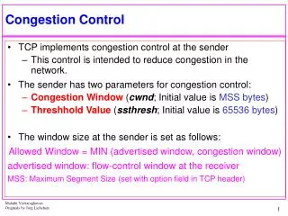
14. TCP Congestion Control • TCP-sender maintains three variables • cwnd– congestion window • rcv_win– receiver advertised window • ssthresh– slow start threshold (used to update cwnd, intuitively ssthresh is a rough estimate of the knee point) • send_win = min (rcv_win, cwnd)

15. TCP Tahoe • implements • slow start • congestion avoidance • fast retransmit algorithm

16. Slow Start (Simplified) • (initially) cwnd =1*Max Segment Size (MSS) • each time an ACK received for a segment cwnd += 1* MSS (exponential growth of cwnd !) • if loss (i.e. timeout), cwnd = 1*MSS again

17. Congestion Avoidance (Simplified) • for each ACK received cwnd += ( MSS*MSS/ cwnd)  approximation of increasing the cwnd by 1*MSS per RTT (additive increase). • if loss(i.e. timeout), cut the cwnd by half (multiplicative decrease).

18. Slow Start & Congestion Avoidance • initally: • cnwd = 1*MSS, ssthresh = very high • if a new ACK comes: • - if cnwd < ssthresh update cwnd according to slow start • if cwnd >= ssthresh  update cnwd according to congestion avoidance • if timeout (i.e. loss) : • - ssthresh = send_win/2; • - cwnd = 1*MSS (initial) ssthresh cwnd timeout (loss) ssthresh time slow start – in green congestion avoidance – in blue

19. cwnd = 1 Example: Slow Start/Congestion Avoidance cwnd = 2 assume (initial) ssthresh = 8*MSS cwnd = 4 cnwd = 8 ssthresh Eight TCP-PDUs Eight ACKs cwnd = 9 nine TCP-PDUs nineACKs cwnd = 10 ten TCP-PDUs ten ACKs cwnd = 11

20. segment 1 cwnd = 1 Fast Retransmit ACK 1 • sender receives 3 dupACKS  sender infers that the segment is lost sender doesn’t wait for timeout  sender re-sends the segment immediately! cwnd = 2 segment 2 segment 3 ACK 2 ACK 3 cwnd = 4 segment 4 segment 5 segment 6 segment 7 ACK 3 3 duplicate ACKs ACK 3 ACK 3 segment 4 fast-retransmit of segment 4

21. TCP Versions: Tahoe fast-retransmit after fast-retransmit sshtresh = send_win/2; cnwd = 1*MSS ; i.e. sender goes back to slow-start ! X Sequence No data ack Time

22. TCP Reno • implements • slow start • congestion avoidance • fast retransmit algorithm & fast recovery

23. Fast Recovery cwnd (initial) ssthresh intuition:receipt of dupACKs tells to the sender that the receiver is still getting new segments, i.e. there is still data flow between sender and receiver  then why sender goes back to slow start after fast retransmit fast-retransmit timeout fast-retransmit new ACK new ACK Time Slow Start Congestion Avoidance “inflating” cwnd with dupACKs “deflating” cwnd with a new ACK

24. Fast Re-transmit & Fast Recovery • sender does the following after receiving 3 dupACKS: 1. sets sshresh = send_win/2 2. retransmits the lost segment 3. sets cwnd = sshthresh + 3*MSS 4. for each dupACK received cwnd += 1*MSS (“inflating” cwnd) 5. if a newACK arrives cwnd = sshresh (value in step 1) (“deflating” cwnd) , and exit fast recovery . • remember: if sender times out, ssthresh = send_win/2, cnwd =1 ! (that is go back to slow start again!)

25. TCP New Reno • implements • slow start • congestion avoidance • fast retransmit &modified fast recovery

26. Modified Fast Recovery TCP Reno – with multiple losses within the same window • motivation: fast recovery (as in Reno) can not recover from multiple losses within the same window efficiently. Sequence No X X X X Now what ? - timeout data ack Time

27. NewReno Sequence No X X X Now what ? – partial ack recovery X data ack Time

28. Modifications to fast recovery • partial ACKs (i.e. the ACK that acks some but not all the packets that were outstanding at the start of fast recovery) : indications of multiple losses • if partial ACK received, re-transmit the next lost segment immediately (whereas in Reno, partial ACKs take TCP out of fast recovery). • sender remains in fast recovery until all data outstanding when fast recovery was initiated is acked.

29. Explicit Congestion Notification (ECN) • Current congestion indication • Use packet drop to indicate congestion • Sources infer congestion implicitly from timeout or triple duplicate ACKs • ECN [IETF RFC2481, 1999] • To give less packet drop and better performance • Uses packet marking rather than dropping • Reduces long timeout and retransmission • Needs cooperation between sources and network • Sources must indicate that they are ECN-capable • Sources and receivers must agree to use ECN • Receiver must inform sources of ECN marks • Sources must react to marks just like losses

30. ECN - 2 • Needs additional flags in TCP header and IP header • In IP header: ECT and CE • ECN Capable Transport (ECT): • Set by sources on all packets to indicate ECN-capability • Congestion Experienced (CE): • Set by routers as a (congestion) marking (instead of dropping) • In TCP header: ECE and CWR • Echo Congestion Experienced (ECE): • When a receiver sees CE, sets ECE on all packets until CWR is received • Congestion Window Reduced (CWR): • Set by a source to indicate that ECE was received and the window size was adjusted (reduced)

31. ECT CE ECT CE 1 0 1 1 IP Header 1 TCP Header 0 0 2 CWR CWR 1 ACK TCP Header ECN-Echo 3 TCP Header 1 CWR 4 Source Router Destination ECN - 3

32. Active Queue Management (AQM) - 1 • Performance Degradation in current TCP Congestion Control • Multiple packet loss • Low link utilization • Congestion collapse • The role of the router becomes important • Control congestion effectively in networks • Allocate bandwidth fairly

33. AQM - 2 • Problems with current router algorithm • Use FIFO based tail-drop (TD) queue management • Two drawbacks with TD: lock-out, full-queue • Lock-out: a small number of flows monopolize usage of buffer capacity • Full-queue: The buffer is always full (high queueing delay) • Possible solution: AQM • Definition: A group of FIFO based queue management mechanisms to support end-to-end congestion control in the Internet

34. AQM - 3 • Goals of AQM • Reducing the average queue length: • Decreasing end-to-end delay • Reducing packet losses: • More efficient resource allocation • Methods: • Drop packets before buffer becomes full • Use (exponentially weighted) average queue length as an congestion indicator • Examples: RED, BLUE, ARED, SRED, FRED,….

35. RED-Introduction Main idea::to provide congestion control at the router for TCP flows. • RED Algorithm Goals • The primary goal is to provide congestion avoidance by controlling the average queue size such that the router stays in a region of low delay and high throughput. • To avoid global synchronization (e.g., in Tahoe TCP). • To control misbehaving users (this is from a fairness context). • To seek a mechanism that is not biased against bursty traffic.

36. RED-Definitions • congestion avoidance –when impending congestion is indicated, take action to avoid congestion. • incipient congestion– congestion that is beginning to be apparent. • need to notify connections of congestion at the router by either marking thepacket [ECN] or dropping the packet {This assumes a drop is an implied signal to the source host.}

37. RED-Previous Work • Drop Tail • Random Drop • Early Random Drop • Source Quench messages • DECbit scheme

38. RED-Drop Tail Router • FIFO queueing mechanism that drops packets when the queue overflows. • Introduces global synchronization when packets are dropped from several connections.

39. RED-Random Drop Router • When a packet arrives and the queue is full, randomly choose a packet from the queue to drop.

40. RED-Early Random Drop Router ? Drop level • If the queue length exceeds a drop level, then the router drops each arriving packet with a fixed drop probability. • Reduces global synchronization • Does not control misbehaving users (UDP)

41. RED-Source Quench messages • Router sends source quenchmessages back to source before queue reaches capacity. • Complex solution that gets router involved in end-to-end protocol.

42. RED-DECbit scheme • Uses a congestion-indication bit in packet header to provide feedback about congestion. • Average queue length is calculated for last (busy + idle) period plus current busy period. • When average queue length exceeds one, set congestion-indicator bit in arriving packet’s header. • If at least half of packets in source’s last window have the bit set, decrease the congestion window exponentially.

43. RED Algorithm for each packet arrival calculate the average queue size avg if minth <= avg < maxth calculate the probability pa with probability pa: mark the arriving packet else if maxth <= avg mark the arriving packet

44. REDdrop probability (pa ) pb = maxpx (avg - minth)/(maxth - minth) [1] where pa = pb/ (1 - count x pb) [2] Note: this calculation assumes queue size is measured in packets. If queue is in bytes, we need to add [1.a] between [1] and [2] pb = pbx PacketSize/MaxPacketSize [1.a]

45. avg - average queue length avg = (1 –wq)x avg + wqx q whereq is the newly measured queue length. This exponential weighted moving average is designed such that short-term increases in queue size from bursty traffic or transient congestion do not significantly increase average queue size.

46. RED/ECN Router Mechanism 1 Dropping/Marking Probability maxp 0 Minth Queue Size Maxth AverageQueue Length

47. RED parameter settings • wq suggest 0.001 <= wq <= 0.0042 authors use wq = 0.002 for simulations • minth, maxthdepend on desired average queue size • bursty traffic  increase minthto maintain link utilization. • maxth depends on the maximum average delay allowed. • RED is most effective when average queue size is larger than typical increase in calculated queue size in one round-trip time. • “parameter setting rule of thumb”:maxthat least twice minth . However, maxth = 3 times minthis used in some of the experiments shown.

48. packet-marking probability • goal: To uniformly spread out the marked packets. This reduces global synchronization. • Method 1: geometric random variable • each packet marked with probability pb • Method 2: uniform random variable • marking probability is pb/ (1 - count x pb) where count is the number of unmarked packets arrived since last marked packet.

49. Method 1: geometric p = 0.02 Method 2: uniform Result :: marked packets more clustered for method 1  uniform is better at eliminating “bursty drops”

50. Setting maxp • “RED performs best when packet-marking probability changes fairly slowly as the average queue size changes.” • This is a stability argument in that the claim is that RED with small maxpwill reduce oscillations in avgand actual marking probability. • They recommend that maxpnever be greater than 0.1 {This is not a robust recommendation}.