Hardware, Software, Quality Assessment
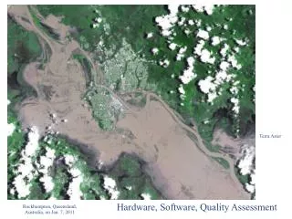
Terra Aster. Hardware, Software, Quality Assessment. Rockhampton , Queensland, Australia, on Jan. 7, 2011. Computer Systems and Peripheral Devices in A Typical Digital Image Processing Laboratory. Image Processing System Hardware /Software Considerations.

Hardware, Software, Quality Assessment
E N D
Presentation Transcript
Terra Aster Hardware, Software, Quality Assessment Rockhampton, Queensland, Australia, on Jan. 7, 2011
Computer Systems and Peripheral Devices in A Typical Digital Image Processing Laboratory
Image Processing System Hardware /Software Considerations • Number and speed of Central Processing Unit(s) (CPU) • Operating system (e.g., Microsoft Windows; UNIX, Linux, Macintosh) • Amount of random access memory (RAM) • Number of image analysts that can use the system at one time and mode of operation (e.g., interactive or batch) • Serial or parallel image processing • Arithmetic coprocessor or array processor • Software compiler(s) (e.g., C++, Visual Basic, Java)
Image Processing System Hardware /Software Considerations • Type of mass storage (e.g., hard disk, CD-ROM, DVD) and amount (e.g., gigabytes) • Monitor display spatial resolution (e.g., 1024 768 pixels) • Monitor color resolution (e.g., 24-bits of image processing video memory yields 16.7 million displayable colors) • Input devices (e.g., optical-mechanical drum or flatbed scanners, area array digitizers) • Output devices (e.g., CD-ROM, CD-RW, DVD-RW, film-writers, line plotters, dye sublimation printers) • Networks (e.g., local area, wide area, Internet)
Operating Systems • The difference between a single-user operating system and a network operating system is the latter’s multi-user capability. • Microsoft Windows XP (home edition) and the Macintosh OS are single-user operating systems designed for one person at a desktop computer working independently. • Various Microsoft Windows, UNIX, and Linux network operating systems are designed to manage multiple user requests at the same time and complex network security.
Image Processing System Functions * Preprocessing (Radiometric and Geometric) * Display and Enhancement * Information Extraction * Photogrammetric Information Extraction * Metadata and Image/Map Lineage Documentation * Image and Map Cartographic Composition * Geographic Information Systems (GIS) * Integrated Image Processing and GIS * Utilities
Selected Commercial and Public Digital Image Processing Systems Jensen, 2009
Selected Commercial and Public Digital Image Processing Systems
Selected Commercial and Public Digital Image Processing Systems
Major Commercial Digital Image Processing Systems • Leica’ ERDAS, ER Mapper, and Photogrammetry Suite • - ENVI • - IDRISI • PCI Geomatica • DefinenseCognition
Major Public Digital Image Processing Systems • - GRASS • MultiSpec (LARS Purdue University - hyperspectral) • VIPER tools (UCSB - hyperspectral) • C-Coast • Adobe Photoshop
Image Quality Assessment & Statistical Evaluation • Many remote sensing datasets contain high-quality, accurate data. Unfortunately, sometimes error (or noise) is introduced into the remote sensor data by: • the environment (e.g., atmospheric scattering), • random or systematic malfunction of the remote sensing • system (e.g., an uncalibrated detector creates striping), or • improper airborne or ground processing of the remote sensor • data prior to actual data analysis (e.g., inaccurate analog-to- • digital conversion).
Remote Sensing Sampling Theory A population is an infinite or finite set of elements. An infinite population could be all possible images that might be acquired of the Earth in 2005. All Landsat 7 ETM+ images of Charleston, S.C. in 2005 is a finite population. A sample is a subset of the elements taken from a population used to make inferences about certain characteristics of the population. For example, we might decide to analyze a June 1, 2008, Landsat image of Charleston. If observations with certain characteristics are systematically excluded from the sample either deliberately or inadvertently (such as selecting images obtained only in the summer), it is a biased sample. Sampling error is the difference between the true value of a population characteristic and the value of that characteristic inferred from a sample.
Remote Sensing Sampling Theory • Large samples drawn randomly from natural populations usually produce a symmetrical frequency distribution. Most values are clustered around some central value, and the frequency of occurrence declines away from this central point. A graph of the distribution appears bell-shaped and is called a normal distribution. • Many statistical tests used in the analysis of remotely sensed data assume that the brightness values recorded in a scene are normally distributed. Unfortunately, remotely sensed data may not be normally distributed and the analyst must be careful to identify such conditions. In such instances, nonparametric statistical theory may be preferred.
Common Symmetric and Skewed Distributions in Remotely Sensed Data
Histogram of A Single Band of Landsat Thematic Mapper Data of Charleston, SC
Viewing Individual Pixels • Viewing individual pixel brightness values in a remotely sensed image is one of the most useful methods for assessing the quality and information content of the data. Virtually all digital image processing systems allow the analyst to: • use a mouse-controlled cursor (cross-hair) to identify a geographic location in the image (at a particular row and column or geographic x,y coordinate) and display its brightness value in n bands, • display the individual brightness values of an individual band in a matrix (raster) format.
Remote Sensing Multivariate Statistics Remote sensing research is often concerned with the measurement of how much radiant flux is reflected or emitted from an object in more than one band (e.g., in red and near-infrared bands). It is useful to compute multivariate statistical measures such as covariance and correlation among the several bands to determine how the measurements covary. Later it will be shown that variance–covariance and correlation matrices are used in remote sensing principal components analysis (PCA), feature selection, classification and accuracy assessment.
Remote Sensing Multivariate Statistics The different remote-sensing-derived spectral measurements for each pixel often change together in some predictable fashion. If there is no relationship between the brightness value in one band and that of another for a given pixel, the values are mutually independent; that is, an increase or decrease in one band’s brightness value is not accompanied by a predictable change in another band’s brightness value. Because spectral measurements of individual pixels may not be independent, some measure of their mutual interaction is needed. This measure, called the covariance, is the joint variation of two variables about their common mean.
Correlation between Multiple Bands of Remotely Sensed Data If we square the correlation coefficient (rkl), we obtain the sample coefficient of determination (r2), which expresses the proportion of the total variation in the values of “band l” that can be accounted for or explained by a linear relationship with the values of the random variable “band k.” Thus a correlation coefficient (rkl) of 0.70 results in an r2 value of 0.49, meaning that 49% of the total variation of the values of “band l” in the sample is accounted for by a linear relationship with values of “band k”.