Turbulence
Turbulence . 14 April 2003 Astronomy G9001 - Spring 2003 Prof. Mordecai-Mark Mac Low. General Thoughts. Turbulence often identified with incompressible turbulence only More general definition needed (V ázquez-Semadeni 1997) Large number of degrees of freedom

Turbulence
E N D
Presentation Transcript
Turbulence 14 April 2003 Astronomy G9001 - Spring 2003 Prof. Mordecai-Mark Mac Low
General Thoughts • Turbulence often identified with incompressible turbulence only • More general definition needed (Vázquez-Semadeni 1997) • Large number of degrees of freedom • Different modes can exchange energy • Sensitive to initial conditions • Mixing occurs
Incompressible Turbulence • Incompressible Navier-Stokes Equation • No density fluctuations: • No magnetic fields, cooling, gravity, other ISM physics advective term (nonlinear) viscosity
Dimensional Analysis • Strength of turbulence given by ratio of advective to dissipative terms, known as Reynold’s number • Energy dissipation rate
Lesieur 1997 Dissipation
Fourier Power Spectrum • Homogeneous turbulence can be considered in Fourier space, to look at structure at different length scales L = 2π/k • Incompressible turbulent energy is just |v|2 • E(k) is the energy spectrum defined by • Energy spectrum is Fourier transform of auto-correlation function
Kolmogorov-Obukhov Cascade • Energy enters at large scales and dissipates at small scales, where 2v most important • Reynold’s number high enough for separation of scales between driving and dissipation • Assume energy transfer only occurs between neighboring scales (Big whirls have little whirls, which feed on their velocity, and little whirls have lesser whirls, and so on to viscosity - Richardson) • Energy input balances energy dissipation • Then energy transfer rate ε must be constant at all scales, and spectrum depends on k and ε.
Compressibility • Again examining the Navier-Stokes equation, we can estimate isothermal density fluctuations ρ = cs-2P • Balance pressure and advective terms: • Flow no longer purely solenoidal (v 0). • Compressible and rotational energy spectra distinct • Compressible spectrum Ec(k) ~ k-2: Fourier transform of shocks
Some special cases • 2D turbulence • Energy and enstrophy cascades reverse • Energy cascades up from driving scale, so large-scale eddies form and survive • Planetary atmospheres typical example • Burgers turbulence • Pressure-free turbulence • Hypersonic limit • Relatively tractable analytically • Energy spectrum E(k) ~ k-2
What is driving the turbulence? • Compare energetics from the different suggested mechanisms (Mac Low & Klessen 2003, Rev. Mod. Phys., on astro-ph) • Normalize to solar circle values in a uniform disk with Rg =15 kpc, and scale height H = 200 pc • Try to account for initial radiative losses when necessary
Mechanisms • Gravitational collapse coupled to shear • Protostellar winds and jets • Magnetorotational instabilities • Massive stars • Expansion of H II regions • Fluctuations in UV field • Stellar winds • Supernovae
Protostellar Outflows • Fraction of mass accreted fwis lost in jet or wind. Shu et al. (1988) suggest fw ~ 0.4 • Mass is ejected close to star, where • Radiative cooling at wind termination shock steals energy ηwfrom turbulence. Assume momentum conservation (McKee 89),
Outflow energy input • Take the surface density of star formation in the solar neighborhood (McKee 1989) • Then energy from outflows and jets is
Magnetorotational Instabilities • Application of Balbus-Hawley (1992,1998) instabilities to galactic disk by Sellwood & Balbus (1999) MMML, Norman, Königl, Wardle 1995
MRI energy input • Numerical models by Hawley, Gammie & Balbus (1995) suggest Maxwell stress tensor • Energy input , so in the Milky Way,
Gravitational Driving • Local gravitational collapse cannot generate enough turbulence to delay further collapse beyond a free-fall time (Klessen et al. 98, Mac Low 99) • Spiral density waves drive shocks/hydraulic jumps that do add energy to turbulence (Lin & Shu, Roberts 69, Martos & Cox). • However, turbulence also strong in irregular galaxies without strong spiral arms
Energy Input from Gravitation • Wada, Meurer, & Norman (2002) estimate energy input from shearing, self-gravitating gas disk (neglecting removal of gas by star formation). • They estimate Newton stress energy input (requires unproven positive correlation between radial, azimuthal gravitational forces)
Stellar Winds • The total energy from a line-driven stellar wind over the lifetime of an early O star can equal the energy of its final supernova explosion. • However, most SNe come from the far more numerous B stars which have much weaker stellar winds. • Although stellar winds may be locally important, they will always be a small fraction of the total energy input from SNe
H II Region Expansion • Total ionizing radiation (Abbott 82) has energy • Most of this energy goes to ionization rather than driving turbulence, however. • Matzner (2002) integrates over H II region luminosity function from McKee & Williams (1997) to find average momentum input
HIIRegion Energy Input • The number of OB associations driving H II regions in the Milky Way is about NOB=650 (from McKee & Williams 1997 with S49>1) • Need to assume vion=10 km s-1, and that star formation lasts for about tion=18.5 Myr, so:
Supernovae • SNe mostly from B stars far from GMCs • Slope of IMF means many more B than O stars • B stars take up to 50 Myr to explode • Take the SN rate in the Milky Way to be roughly σSN=1 SNu (Capellaro et al. 1999), so the SN rate is 1/50 yr • Fraction of energy surviving radiative cooling ηSN ~ 0.1 (Thornton et al. 1998)
Supernova Energy Input • If we distribute the SN energy equally over a galactic disk, • SNe appear hundreds or thousands of times more powerful than all other energy sources
Assignments • Abel, Bryan, & Norman, Science, 295, 93 [This will be discussed after Simon Glover’s guest lecture, sometime in the next several weeks] • Sections 1, 2, and 5 of Klessen & Mac Low 2003, astro-ph/0301093 [to be discussed after my next lecture] • Exercise 6
Piecewise Parabolic Method • Third-order advection • Godunov method for flux estimation • Contact discontinuity steepeners • Small amount of linear artificial viscosity • Described by Colella & Woodward 1984, JCP, compared to other methods by Woodward & Colella 1984, JCP.
Parabolic Advection • Consider the linear advection equation • Zone average values must satisfy • A piecewise continuous function with a parabolic profile in each zone that does so is
Interpolation to zone edges • To find the left and right values aLandaR, compute a polynomial using nearby zone averages. For constant zone widths Δξj • In some cases this is not monotonic, so add: • And similarly for aR,j to force montonicity.
Conservative Form • Euler’s equations in conservation form on a 1D Cartesian grid gravity or other body forces conserved variables fluxes pressure
Godunov method • Solve a Riemann shock tube problem at every zone boundary to determine fluxes
Characteristic averaging • To find left and right states for Riemann problem, average over regions covered by characteristic: max(cs,u) Δt tn+1 tn+1 or tn tn xj xj xj-1 xj+1 xj-1 xj+1 subsonic flow supersonic flow (from left)
Characteristic speeds • Characteristic speeds are not constant across rarefaction or shock because of change in pressure
Riemann problem • A typical analytic solution for pressure (P. Ricker) is given by the root of