Semantics
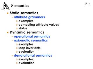
Semantics. In Text: Chapter 3. Outline. Semantics: Attribute grammars (static semantics) Operational Axiomatic Denotational. Static Semantics. CFGs cannot describe all of the syntax of programming languages—context-specific parts are left out

Semantics
E N D
Presentation Transcript
Semantics In Text: Chapter 3
Outline • Semantics: • Attribute grammars (static semantics) • Operational • Axiomatic • Denotational Chapter 3: Syntax and Semantics
Static Semantics • CFGs cannot describe all of the syntax of programming languages—context-specific parts are left out • Static semantics refers to type checking and resolving declarations; has nothing to do with “meaning” in the sense of run-time behavior • Often described using an attribute grammar (AG) (Knuth, 1968) • Basic idea: add to CFG by carrying some semantic information along inside parse tree nodes • Primary value of AGs: • Static semantics specification • Compiler design (static semantics checking) Chapter 3: Syntax and Semantics
Dynamic Semantics • No single widely acceptable notation or formalism for describing semantics • Three common approaches: • Operational • Axiomatic • Denotational Chapter 3: Syntax and Semantics
Operational Semantics • Gives a program's meaning in terms of its implementation on a real or virtual machine • Change in the state of the machine (memory, registers, etc.) defines the meaning of the statement • To use operational semantics for a high-level language, a virtual machine in needed • A pure hardware interpreter is too expensive • A pure software interpreter also has problems: • machine-dependent • Difficult to understand • A better alternative: A complete computer simulation Chapter 3: Syntax and Semantics
Operational Semantics (cont.) • The process: • Identify a virtual machine (an idealized computer) • Build a translator (translates source code to the machine code of an idealized computer) • Build a simulator for the idealized computer • Operational semantics is sometimes called translational semantics, if an existing PL is used in place of the virtual machine Chapter 3: Syntax and Semantics
Operational Semantics Example • Operational semantics could be much lower level: mov i,r1 mov y,r2 jmpifless(r2,r1,out) ... out: ... Chapter 3: Syntax and Semantics
Evaluation of Operational Semantics • Advantages: • May be simple, intuitive for small examples • Good if used informally • Useful for implementation • Disadvantages • Very complex for large programs • Lacks mathematical rigor • Uses: • Vienna Definition Language (VDL) used to define PL/I (Wegner 1972) • Compiler work Chapter 3: Syntax and Semantics
Axiomatic Semantics • Based on formal logic (first order predicate calculus) • Original purpose: formal program verification • Approach: Define axioms or inference rules for each statement type in the language • Such an inference rule allows one to transform expressions to other expressions • The expressions are called assertions, and state the relationships and constraints among variables that are true at a specific point in execution • An assertion before a statement is called a precondition • An assertion following a statement is a postcondition Chapter 3: Syntax and Semantics
Weakest Preconditions • Pre-post form: {P} statement {Q} • A weakest precondition is the least restrictive precondition that will guarantee the postcondition • An example: a := b + 1 {a > 1} • One possible precondition: {b > 10} • Weakest precondition: {b > 0 } Chapter 3: Syntax and Semantics
Program Proofs • Program proof process: • The postcondition for the whole program is the desired results • Work back through the program to the first statement • If the precondition on the first statement is the same as the program spec, the program is correct Chapter 3: Syntax and Semantics
An Axiom for Assignment • An axiom for assignment statements: {Qx->E} x := E {Q} • Substitute E for every x in Q { P? } x := y+1 { x > 0 } P = x > 0 x -> y+1 P = y+1 > 0 P = y 0 • Basically, “undoing” the assignment and solving for y Chapter 3: Syntax and Semantics
Some Inference Rules • The Rule of Consequence: {P} S {Q}, P' => P, Q => Q' {P'} S {Q'} • For a sequence S1;S2 the inference rule is: {P1} S1 {P2}, {P2} S2 {P3} {P1} S1; S2 {P3} Chapter 3: Syntax and Semantics
A Rule for Loops • An inference rule for logical pretest loops: {P} while B do S end {Q} • The inference rule is: {I and B} S {I} {I} while B do S {I and (not B)} • Where I is the loop invariant. Chapter 3: Syntax and Semantics
Loop Invariant Characteristicss I must meet the following conditions: 1. P I (the loop invariant must be true initially) 2. {I} B {I} (evaluation of the Boolean must not change the validity of I) 3. {I and B} S {I} (I is not changed by executing the body of the loop) 4. (I and (not B)) Q (if I is true and B is false, Q is implied) 5. The loop terminates (can be difficult to prove) Chapter 3: Syntax and Semantics
More on Loop Invariants • The loop invariant I is: • A weakened version of the loop postcondition, and • Also the loop’s precondition • I must be: • Weak enough to be satisfied prior to the beginning of the loop, but • when combined with the loop exit condition, it must be strong enough to force the truth of the postcondition Chapter 3: Syntax and Semantics
Finding Loop Invariants • Work backwards through a few iterations and look for a pattern while y <> x do y:= y+1 {y = x} {P?} y := y + 1 {y = x} P = {y = x}y -> y + 1 = {y = x – 1} —last iteration {P?} y := y + 1 {y = x - 1} P = {y = x-1}y -> y + 1 = {y = x – 2} —next to last Chapter 3: Syntax and Semantics
Finding Invariants (cont.) • By extension, we get I = { y < x } • When we factor in that the loop may not be executed even once (when y = x), we get I = { y x } • This also satisfies loop termination, so • P = I = {y x} Chapter 3: Syntax and Semantics
Is I a Loop Invariant? • Does {y x} satisfy the 5 conditions? (1) {y x} {y x} ? (2) if {y x} and y <> x is then evaluated, is {y x} still true? (3) if {y x} and y <> x are true and then y := y+1 is executed, is {y x} true? (4) does {y x} and {y = x} {y = x}? • Can you argue convincingly that the program segment terminates? Chapter 3: Syntax and Semantics
A Harder Loop Invariant Example {P} while y < x + 1 do y := y + 1 {y>5} {y > 5}y -> y + 1 y > 4 {y > 4}y -> y + 1 y > 3 etc. • Tells us nothing about x because x is not in Q {y > 5} • What else can we do? Chapter 3: Syntax and Semantics
Using Loop Criterion 4 • Try guessing invariant using criterion 4: • {I and (not B)} Q • I? and y x + 1 y > 5 • I? and y > x y > 5 • any x 5 satisfies implication • so . . . let I = {x 5} • Do the 4 Axioms hold? Chapter 3: Syntax and Semantics
Evaluation of Axiomatic Semantics • Advantages • Can be very abstract • May be useful in proofs of correctness • Solid theoretical foundations • Disadvantages • Predicate transformers are hard to define • Hard to give complete meaning • Does not suggest implementation • Uses of Axiomatic Semantics • Semantics of Pascal • Reasoning about correctness Chapter 3: Syntax and Semantics
Denotational Semantics • Based on recursive function theory • The most abstract semantics description method • Originally developed by Scott and Strachey (1970) • Key idea: Define a function that maps a program (a syntactic object) to its meaning (a semantic object) Chapter 3: Syntax and Semantics
Denotational vs. Operational • Denotational semantics is similar to high-level operational semantics, except: • Machine is gone • Language is mathematics (lamda calculus) • The difference between denotational and operational semantics: • In operational semantics, the state changes are defined by coded algorithms for a virtual machine • In denotational semantics, they are defined by rigorous mathematical functions Chapter 3: Syntax and Semantics
Denotational Specification Process 1. Define a mathematical object for each language entity 2. Define a function that maps instances of the language entities onto instances of the corresponding mathematical objects Chapter 3: Syntax and Semantics
Program State • The meaning of language constructs are defined only by the values of the program's variables • The state of a program is the values of all its current variables, plus input and output state s = {<i1, v1>, <i2, v2>, …, <in, vn>} • Let VARMAP be a function that, when given a variable name and a state, returns the current value of the variable: VARMAP(ij, s) = vj Chapter 3: Syntax and Semantics
Example: Decimal Numbers <digit> -> 0 | 1 | 2 | 3 | 4 | 5 | 6 | 7 | 8 | 9 <dec_num> -> <digit> | <dec_num><digit> • Mdec('0') = 0, Mdec('1') = 1, …, Mdec('9') = 9 • Mdec(<dec_num>) = case <dec_num> of <digit> Mdec(<digit>) <dec_num><digit> 10 Mdec(<dec_num>) + Mdec(<digit>) Chapter 3: Syntax and Semantics
Expressions • Me(<expr>, s) = case <expr> of <dec_num> Mdec(<dec_num>, s) <var> VARMAP(<var>, s) <binary_expr> if (<binary_expr>.<operator> = ‘+’) then Me(<binary_expr>.<left_expr>, s) + Me(<binary_expr>.<right_expr>, s) else Me(<binary_expr>.<left_expr>, s) Me(<binary_expr>.<right_expr>, s) Chapter 3: Syntax and Semantics
Statement Basics • The meaning of a single statement executed in a state s is a new state s’ (that reflects the effects of the statement) Mstmt( Stmt , s) = s’ • For a sequence of statements: Mstmt( Stmt1; Stmt2 , s) = Mstmt( Stmt2 , Mstmt( Stmt1 , s)) or Mstmt( Stmt1; Stmt2 , s) = S’’ where s’ = Mstmt( Stmt1 , s) s’’ = Mstmt( Stmt2 , s’) Chapter 3: Syntax and Semantics
Assignment Statements • Ma(x := E, s) = s’ = {<i1’, v1’>, <i2’, v2’>, ..., <in’,vn’>}, where for j = 1, 2, ..., n, vj’ = VARMAP(ij, s) if ij x vj’ = Me(E, s) if ij = x Chapter 3: Syntax and Semantics
Sequence of Statements } x := 5; y := x + 1; P1 P write(x * y); } P2 Initial state s0 = <mem0, i0, o0> Mstmt( P , s) = Mstmt( P1 , Mstmt( x := 5 , s)) s1 = <mem1,i1,o1> where s1 VARMAP(x, s1) = 5 VARMAP(z, s1) = VARMAP(z, s0) for all z x i1 = i0, o1 = o0 } Chapter 3: Syntax and Semantics
Sequence of Statements (cont.) Mstmt( P1 , s1) = Mstmt( P2 , Mstmt( y := x + 1 , s1)) s2 s2 = <mem2, i2, o2> where VARMAP(y, s2) = Me( x + 1 , s1) = 6 VARMAP(z, s2) = VARMAP(z, s1) for all z y i2 = i1 o2 = o1 Chapter 3: Syntax and Semantics
Sequence of Statements (cont.) Mstmt( P2 , s2) = Mstmt( write (x * y) , s2) = s3 s3 = <mem3, i3, o3> where VARMAP(z, s3) = VARMAP(z, s2) for all z i3 = i2 o3 = o2 • Me( x * y , s2) = o2 • 30 Chapter 3: Syntax and Semantics
Sequence of Statements (concl.) So, Mstmt( P , s0) = s3 = <mem3, i3, o3 > where VARMAP(y, s3) = 6 VARMAP(x, s3) = 5 VARMAP(z, s3) = VARMAP(z, s0) for all z x, y i3 = i0 o3 = o0 • 30 Chapter 3: Syntax and Semantics
Logical Pretest Loops • The meaning of the loop is the value of the program variables after the loop body has been executed the prescribed number of times, assuming there have been no errors • In essence, the loop has been converted from iteration to recursion, where the recursive control is mathematically defined by other recursive state mapping functions • Recursion, when compared to iteration, is easier to describe with mathematical rigor Chapter 3: Syntax and Semantics
Logical Pretest Loops (cont.) • Ml(while B do L, s) = if Mb(B, s) = false then s else Ml(while B do L, Ms(L, s)) Chapter 3: Syntax and Semantics
Evaluation of Denotational Semantics • Advantages: • Compact & precise, with solid mathematical foundation • Provides a rigorous way to think about programs • Can be used to prove the correctness of programs • Can be an aid to language design • Has been used in compiler generation systems • Disadvantages • Requires mathematical sophistication • Hard for programmer to use • Uses • Semantics for Algol-60, Pascal, etc. • Compiler generation and optimization Chapter 3: Syntax and Semantics
Summary • Each form of semantic description has its place: • Operational • Informal descriptions • Compiler work • Axiomatic • Reasoning about particular properties • Proofs of correctness • Denotational • Formal definitions • Provably correct implementations Chapter 3: Syntax and Semantics