Download
1 / 75
790 likes | 1.3k Views
CHAPTER 9 ESTIMATING THE VALUE OF A PARAMETER USING CONFIDENCE INTERVAL. 9.1 confidence interval for the population mean when the population standard deviation is known. 9.1 Objectives. Compute a point estimate of the population mean

E N D
CHAPTER 9ESTIMATING THE VALUE OF A PARAMETER USING CONFIDENCE INTERVAL
9.1 confidence interval for the population mean when the population standard deviation is known
9.1 Objectives • Compute a point estimate of the population mean • Construct and interpret a confidence interval for the population mean assuming that the population standard deviation is known • Understand the role of margin of error in constructing the confidence interval • Determine the sample size necessary for estimating the population mean within a specified margin of error
Objective 1 • Compute a Point Estimate of the Population Mean A point estimate is the value of a statistic that estimates the value of a parameter. For example, the sample mean, , is a point estimate of the population mean .
Parallel Example 1: Computing a Point Estimate Pennies minted after 1982 are made from 97.5% zinc and 2.5% copper. The following data represent the weights (in grams) of 17 randomly selected pennies minted after 1982. 2.46 2.47 2.49 2.48 2.50 2.44 2.46 2.45 2.49 2.47 2.45 2.46 2.45 2.46 2.47 2.44 2.45 Treat the data as a simple random sample. Estimate the population mean weight of pennies minted after 1982.
Solution The sample mean is The point estimate of is grams.
Objective 2 • Construct and Interpret a Confidence Interval for the Population Mean
A confidence interval for an unknown parameter consists of an interval of values. The level of confidence represents the expected proportion of intervals that will contain the parameter if a large number of different samples is obtained. The level of confidence is denoted (1-)·100%.
For example, a 95% level of confidence (=0.05) implies that if 100 different confidence intervals are constructed, each based on a different sample from the same population, we will expect 95 of the intervals to contain the parameter and 5 to not include the parameter.
Confidence interval estimates for the population mean are of the form Point estimate ± margin of error. • The margin of error of a confidence interval estimate of a parameter is a measure of how accurate the point estimate is.
The margin of error depends on three factors: • Level of confidence: As the level of confidence increases, the margin of error also increases. • Sample size: As the size of the random sample increases, the margin of error decreases. • Standard deviation of the population: The more spread there is in the population, the wider our interval will be for a given level of confidence.
The shape of the distribution of all possible sample means will be normal, provided the population is normal or approximately normal, if the sample size is large (n≥30), with • mean • and standard deviation .
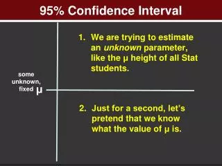
Interpretation of a Confidence Interval A (1-)·100% confidence interval indicates that, if we obtained many simple random samples of size n from the population whose mean, , is unknown, then approximately (1-)·100% of the intervals will contain . For example, if we constructed a 99% confidence interval with a lower bound of 52 and an upper bound of 71, we would interpret the interval as follows: “We are 99% confident that the population mean, , is between 52 and 71.”
Constructing a (1- )·100%Confidence Interval for , Known Suppose that a simple random sample of size n is taken from a population with unknown mean, , and known standard deviation . A (1-)·100% confidence interval for is given by where is the critical Z-value. Note: The sample size must be large (n≥30) or the population must be normally distributed. Lower Upper Bound: Bound:
Parallel Example 3: Constructing a Confidence Interval Construct a 99% confidence interval about the population mean weight (in grams) of pennies minted after 1982. Assume =0.02 grams. 2.46 2.47 2.49 2.48 2.50 2.44 2.46 2.45 2.49 2.47 2.45 2.46 2.45 2.46 2.47 2.44 2.45
Lower bound: = • Upper bound: = We are 99% confident that the mean weight of pennies minted after 1982 is between and grams.
Objective 3 • Understand the Role of the Margin of Error in Constructing a Confidence Interval
The margin of error, E, in a (1-)·100% confidence interval in which is known is given by where n is the sample size. Note: We require that the population from which the sample was drawn be normally distributed or the samples size n be greater than or equal to 30.
Parallel Example 5: Role of the Level of Confidence in the Margin of Error Construct a 90% confidence interval for the mean weight of pennies minted after 1982. Comment on the effect that decreasing the level of confidence has on the margin of error.
Lower bound: = • Upper bound: = We are 90% confident that the mean weight of pennies minted after 1982 is between and grams.
Notice that the margin of error decreased from 0.012 to 0.008 when the level of confidence decreased from 99% to 90%. The interval is therefore wider for the higher level of confidence.
Parallel Example 6: Role of Sample Size in the Margin of Error Suppose that we obtained a simple random sample of pennies minted after 1982. Construct a 99% confidence interval with n=35. Assume the larger sample size results in the same sample mean, 2.464. The standard deviation is still =0.02. Comment on the effect increasing sample size has on the width of the interval.
Lower bound: = • Upper bound: = We are 99% confident that the mean weight of pennies minted after 1982 is between and grams.
Notice that the margin of error decreased from 0.012 to 0.009 when the sample size increased from 17 to 35. The interval is therefore narrower for the larger sample size.
Objective 4 • Determine the Sample Size Necessary for Estimating the Population Mean within a Specified Margin of Error
Determining the Sample Size n The sample size required to estimate the population mean, , with a level of confidence (1-)·100% with a specified margin of error, E, is given by where n is rounded up to the nearest whole number.
Parallel Example 7: Determining the Sample Size Back to the pennies. How large a sample would be required to estimate the mean weight of a penny manufactured after 1982 within 0.005 grams with 99% confidence? Assume =0.02.
=0.02 • E=0.005 Rounding up, we find n= .
9.2 confidence interval for the population mean when the population standard deviation is unknown
9.2 Objectives • Know the properties of Student’s t-distribution 2. Determine t-values 3. Construct and interpret a confidence interval for a population mean when the standard deviation is unknown.
Objective 1 • Know the Properties of Student’s t-Distribution
Student’s t-Distribution Suppose that a simple random sample of size n is taken from a population. If the population from which the sample is drawn follows a normal distribution, the distribution of follows Student’s t-distribution with n-1 degrees of freedom where is the sample mean and s is the sample standard deviation.
Parallel Example 1: Comparing the Standard Normal Distribution to the t-Distribution Using Simulation • Obtain 1,000 simple random samples of size n=5 from a normal population with =50 and =10. • Determine the sample mean and sample standard deviation for each of the samples. • Compute and for each sample. • Draw a histogram for both z and t.
Histogram for z Histogram for t
CONCLUSIONS: • The histogram for z is symmetric and bell-shaped with the center of the distribution at 0 and virtually all the rectangles between -3 and 3. In other words, z follows a standard normal distribution. • The histogram for t is also symmetric and bell-shaped with the center of the distribution at 0, but the distribution of t has longer tails (i.e., t is more dispersed), so it is unlikely that t follows a standard normal distribution. The additional spread in the distribution of t can be attributed to the fact that we use s to find t instead of . Because the sample standard deviation is itself a random variable (rather than a constant such as ), we have more dispersion in the distribution of t.
Properties of the t-Distribution • The t-distribution is different for different degrees of freedom. • The t-distribution is centered at 0 and is symmetric about 0. • The area under the curve is 1. The area under the curve to the right of 0 equals the area under the curve to the left of 0 equals 1/2. • As t increases without bound, the graph approaches, but never equals, zero. As t decreases without bound, the graph approaches, but never equals, zero.
The area in the tails of the t-distribution is a little greater than the area in the tails of the standard normal distribution, because we are using s as an estimate of , thereby introducing further variability into the t- statistic. • As the sample size n increases, the density curve of t gets closer to the standard normal density curve. This result occurs because, as the sample size n increases, the values of s get closer to the values of , by the Law of Large Numbers.
Objective 2 • Determine t-Values
Parallel Example 2: Finding t-values Find the t-value such that the area under the t-distribution to the right of the t-value is 0.2 assuming 10 degrees of freedom. That is, find t0.20 with 10 degrees of freedom.
Solution The figure to the left shows the graph of the t-distribution with 10 degrees of freedom. The unknown value of t is labeled, and the area under the curve to the right of t is shaded. The value of t0.20with 10 degrees of freedom is 0.8791.
Objective 3 • Construct and Interpret a Confidence Interval for a Population Mean
Constructing a (1-)100% Confidence Interval for , Unknown Suppose that a simple random sample of size n is taken from a population with unknown mean and unknown standard deviation . A (1-)100% confidence interval for is given by Lower Upper bound: bound: Note: The interval is exact when the population is normally distributed. It is approximately correct for nonnormal populations, provided that n is large enough.
Parallel Example 3: Constructing a Confidence Interval about a Population Mean The pasteurization process reduces the amount of bacteria found in dairy products, such as milk. The following data represent the counts of bacteria in pasteurized milk (in CFU/mL) for a random sample of 12 pasteurized glasses of milk. Data courtesy of Dr. Michael Lee, Professor, Joliet Junior College. Construct a 95% confidence interval for the bacteria count.
NOTE: Each observation is in tens of thousand. So, 9.06 represents 9.06 x 10⁴.
Lower bound: Upper bound: The 95% confidence interval for the mean bacteria count in pasteurized milk is (3.52, 9.30).
9.3 Objectives • Obtain a point estimate for the population proportion • Construct and interpret a confidence interval for the population proportion • Determine the sample size necessary for estimating a population proportion within a specified margin of error
Objective 1 • Obtain a point estimate for the population proportion
A point estimate is an unbiased estimator of the parameter. The point estimate for the population proportion is where x is the number of individuals in the sample with the specified characteristic and n is the sample size.