Review - Confidence Interval
This review discusses the concept of confidence intervals, particularly focusing on their application in social science research. By examining the normal distribution of variables like officer cynicism, we explore how repeated random samples can yield means that distribute normally. Using z-scores, specifically a z of 1.96, we establish confidence intervals that indicate a 95% certainty that the population mean falls within a specific range. Results from two samples of officers illustrate how to calculate means, variances, and standard deviations, emphasizing the importance of sample size and z-scores in narrowing confidence intervals.

Review - Confidence Interval
E N D
Presentation Transcript
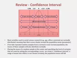
Review - Confidence Interval -1.96 -1.0 0 +1.0 +1.96 • Most variables used in social science research (e.g., age, officer cynicism) are normally distributed, meaning that their scores cluster around the population mean (parameter) • If we take repeated random samples from a normal or near-normal population, the means of these samples will also distribute normally • Placing the mean of a random sample at the center, and specifying the level of certainty that we want by setting the corresponding z score, we create a “confidence interval”, a range of means into which, to our chosen certainty, the population mean will fall 17 pct. of scores 66 pct. 17 pct. of scores 100 percent of scores 2 ½ pct. 95 percent of scores 2 ½ pct.
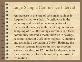
Homework • Two random samples of officers tested for cynicism • For each sample, we needed to specify the confidence interval into which the population parameter (mean of population) will fall, to a 95 percent certainty • In social science research we don’t want to take more than five chances in 100, or 5 percent, of being wrong • Remember that 95 percent of the cases in a normally distributed population fall between a z of -1.96 and +1.96 (meaning that 5 percent will not) • So - always use a z of 1.96
Sample 1 (n=10) Officer Score Mean Diff. Sq. 1 3 2.9 .1 .01 2 3 2.9 .1 .01 3 3 2.9 .1 .01 4 3 2.9 .1 .01 5 3 2.9 .1 .01 6 3 2.9 .1 .01 7 3 2.9 .1 .01 8 1 2.90 1.9 3.61 9 2 2.9 .9 .81 10 5 2.9 2.1 4.41 Sum 8.90 Variance (sum of squares / n-1) s2 .99 Standard deviation (sq. root of variance) s .99
Sample 2 (n=10) Officer Score Mean Diff. Sq. 1 2 2.4 .4 .16 2 1 2.4 1.4 1.96 3 1 2.4 1.4 1.96 4 2 2.4 .4 .16 5 3 2.4 .6 .36 6 3 2.4 .6 .36 7 3 2.4 .6 .36 8 3 2.4 .6 .36 9 4 2.4 1.6 2.56 10 2 2.4 .4 .16 Sum 8.40 Variance (sum of squares / n-1) s2 .93 Standard deviation (sq. root of variance) s .97
Standard error of the mean of the population of patrol officers Estimated difference, due to chance, between the means of repeated random samples (in this example, of 10 patrol officers) and the population parameter (mean of the population) s Sx = ------- ___ n-1 Estimate based on sample 1 = .33 Estimate based on sample 2 = .32
Confidence interval into which the population mean should fall with a 95 percent certainty (probability 5 percent that population parameter - mean - falls outside this range) ci =x +/- z (Sx ) Results based on sample 1: Mean = 2.9 Sx = .33 (z = 1.96) 2.9 +/- .65 Left limit = 2.25 Right limit = 3.55 Results based on sample 2: Mean = 2.4 Sx = .32 (z = 1.96) 2.4 +/- .63 Left limit = 1.77 Right limit = 3.03
Answer for final exam • There will be one word question on the final for each statistical technique covered during the period • Here is the question for confidence interval: • Explain what you would tell the police chief that the confidence interval that you computed actually means • Here is a good answer: • There are ninety-five chances in one-hundred that, based on the mean __(insert variable)___ calculated from a random sample of (insert sample size) officers, the mean for all the officers in the department would fall between _______ and _______.
Review - Confidence Interval z scores -1.96 -1.0 0 +1.0 +1.96 2.25 2.9 3.55 • Our first sample had a mean of 2.9. The second sample mean was 2.4. • We used a z of 1.96, which set the probability that the population mean would fall within our confidence interval at 95 percent • Based on sample 1, there are 95 chances in 100 that the population mean (parameter) falls between 2.25 and 3.55. Or, there are 5 chances in 100 that it doesn’t. • Based on sample 2, there are 95 chances in 100 that the population mean (parameter) falls between 1.77 and 3.03. Or, there are 5 chances in 100 that it doesn’t. Sample 1 1.77 2.4 3.03 Sample 2 2 ½ pct. 95 percent of scores 2 ½ pct.
How to narrow the confidence interval #1 • Increase the probability of being wrong! That is, the chance that the population mean (parameter) actually falls OUTSIDE the calculated range • First, select a smaller z-score. Say, z = 1.0 • According to the z-table, .3413 of cases (34%) fall between the mean and z = 1.0 • So, another 34% of the cases must fall between the mean and z = -1.0 • That’s 68% of the cases. So, 32% of the cases must fall outside this range(68% + 32% = 100%) • This presents a much bigger chance of being wrong than by using a z of 1.96, where only 5% of the cases fall outside the range • In social science research, we always use a z of 1.96 to set confidence intervals, because we don’t want to take a greater than 5 in 100 chance of being wrong ci =x +/- z (Sx ) • Results based on sample 1: • Mean = 2.9 Sx = .33 z = 1.00 • 2.9 +/- .33 Left limit = 2.57 Right limit = 3.23 • Results based on sample 2: • Mean = 2.4 Sx = .32 z = 1.00 • 2.4 +/- .32 Left limit = 2.08 Right limit = 2.72
How to narrow the confidence interval #2 • Increase the sample size! • This lets you use z = 1.96, so that the probability that the population parameter falls within the confidence interval is the social science required 95 percent ci =x +/- z (Sx ) • Increase sample 1 size to 30, and to 100 • To keep things simple, the sum of squares (8.9) was tripled, and also multiplied by 10. The mean (2.9) was kept the same • n = 30 • New sum of squares = 26.7 • s2 (variance) = .92 • s (standard deviation) = .96 • Sx (standard error of the mean) = .18 • z (Sx ) = .35 • Confidence interval = 2.55 3.25 • Old ci was 2.25 3.55 • n = 100 • New sum of squares = 89 • s2 (variance) = .9 • s (standard deviation) = .95 • Sx (standard error of the mean) = .1 • z (Sx ) = .2 • Confidence interval = 2.7 3.1 • Old ci was 2.25 3.55
Diff. Between Means Test • Independent variable is categorical and the dependent variable is continuous • To determine if these variables are associated compare the means of two randomly drawn samples • Is the difference between the means so large that we can reject the null hypothesis (that the difference was produced by chance?) • Must calculate standard error of the difference between means • The difference between all possible pairs of means, due to chance alone • To do so: • Obtain the “pooled sample variance” (for us, half-way between the obtained variances) • Compute the S.E. of the Diff. Between Means • Compute the t-statistic
Pooled sample varianceSp2 Simplified method: midpoint between the two sample variances Sp2 = Standard error of the difference between meansx1 -x2 x1 -x2 = Sp2 ( ) T-Test for significance of the difference between means x1 -x2t = --------------x1 -x2 s21 + s22 2 1 1 n1 n2 +
df = (n1 + n2) - 2 • The result is a ratio • Our obtained difference between means is on top • The predicted difference due to error is on the bottom • The greater our difference, the larger the t • The larger the t, the more likely we are to reject the null hypothesis (see the t-table in the back of the book) • When we reject the null hypothesis, we say that the difference between means is statistically significant, meaning that the samples were not drawn from the same population – we only thought they were x 1 - x 2 _____________________ x 1 - x 2 t =
Class exercise -- Difference Between Means Test H1: Male officers more cynical than females (1 - tailed) H2: Officer gender determines cynicism (2 - tailed) • What is the null hypothesis? • Draw one sample of male officers, one of females • Compute the Standard Error of the Difference Between Means • Perform a t-test • Use the table in the back of the book to check for significance (no more than 5 chances in 100 that the null hypo. is correct) Note: one tailed hypotheses (direction of the effect on the dependent variable is predicted) require a smaller “t” to reach statistical significance than two-tailed hypotheses, where only an effect is predicted, not its direction Discuss homework assignment