Download
1 / 35
350 likes | 461 Views
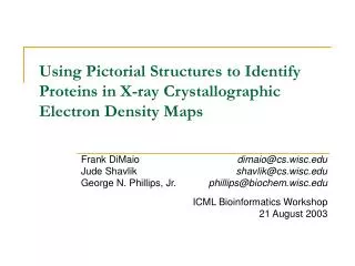
This paper presents a probabilistic approach to trace protein backbones utilizing electron density maps obtained through X-ray crystallography. The method employs a combination of local matching and global consistency algorithms to filter false positives and identify the most probable backbone trace. Through the application of Markov Field Models and belief propagation, we estimate joint probabilities of amino acid positioning while considering structural constraints. We evaluate our method, ACMI, against established algorithms like TEXTAL and Resolve across models with varying density map resolutions.

E N D
A Probabilistic Approach to Protein Backbone Tracing in Electron Density Maps Frank DiMaio, Jude Shavlik Computer Sciences Department George Phillips Biochemistry Department University of Wisconsin – Madison USA Presented at the Fourteenth Conference on Intelligent Systems for Molecular Biology (ISMB 2006), Fortaleza, Brazil, August 7, 2006
X-ray Crystallography FFT X-ray beam ProteinCrystal CollectionPlate ElectronDensity Map (“3D picture”)
Given: Sequence + Density Map Sequence + Electron Density Map
Our Subtask: Backbone Trace Cα Cα Cα Cα
The Unit Cell • 3D density function ρ(x,y,z) provided over unit cell • Unit cell may contain multiple copies of the protein
The Unit Cell • 3D density function ρ(x,y,z) provided over unit cell • Unit cell may contain multiple copies of the protein
Density Map Resolution 2Å 4Å 3Å ARP/wARP (Perrakis et al. 1997) TEXTAL (Ioerger et al. 1999) Resolve (Terwilliger 2002) Our focus
Overview of ACMI (our method) • Local Match • Algorithm searches for sequence-specific 5-mers centered at each amino acid • Many false positives • Global Consistency • Use probabilistic model to filter false positives • Find most probable backbone trace • Global Consistency • Use probabilistic model to filter false positives • Find most probable backbone trace
5-mer Lookup and Cluster …VKHVLVSPEKIEELIKGY… PDB Cluster 1 Cluster 2 NOTE: can be done in precompute step wt=0.67 wt=0.33
5-mer Search • 6D search (rotation + translation) forrepresentative structures in density map • Compute “similarity” • Computed by Fourier convolution (Cowtan 2001) • Use tuneset to convert similarity score to probability
NEG POS match to tuneset Bayes’ rule score distributions probability distribution over unit cell P(5-mer at ui|Map) search density map scores ti (ui) Convert Scores to Probabilities 5-mer representative
In This Talk… • Where we are now For each amino acid in the protein, we have a probability distribution over the unit cell • Where we are headed Find the backbone layout maximizing
Pairwise Markov Field Models • A type of undirected graphical model • Represent joint probabilities as product ofvertexand edge potentials • Similar to (but more general than) Bayesian networks y u1 u2 u3
Protein Backbone Model • Each vertexis an amino acid • Each label is location + orientation • Evidence y is the electron density map • Each vertex (or observational) potentialcomes from the 5-mer matching ALA GLY LYS LEU
Protein Backbone Model ALA GLY LYS LEU • Two types of edge (or structural) potentials • Adjacency constraints ensure adjacent amino acids are ~3.8Å apart and in the proper orientation
Protein Backbone Model ALA GLY LYS LEU • Two types of structural (edge) potentials • Adjacency constraints ensure adjacent amino acids are ~3.8Å apart and in the proper orientation • Occupancy constraints ensure nonadjacent amino acids do not occupy same 3D space
Backbone Model Potential Constraints between adjacent amino acids: = x
Backbone Model Potential Constraints between nonadjacent amino acids:
Backbone Model Potential Observational (“amino-acid-finder”) probabilities
Probabilistic Inference • Want to find backbone layout that maximizes • Exact methods are intractable • Use belief propagation (BP) to approximate marginal distributions
Belief Propagation (BP) • Iterative, message-passing method (Pearl 1988) • A message, , from amino acid i toamino acid j indicates where i expects to find j • An approximation to the marginal (or belief),is given as the product of incoming messages
Belief Propagation Example ALA GLY
Technical Challenges • Representation of potentials • Store Fourier coefficients in Cartesian space • At each location x, store a single orientation r • Speeding up O(N2X2) naïve implementation • X = the unit cell size (# Fourier coefficients) • N = the number of residues in the protein
Speeding Up O(N2X2) Implementation • O(X2) computation for each occupancy message • Each message must integrate over the unit cell • O(X log X) as multiplication in Fourier space • O(N2) messages computed & stored • Approx N-3 occupancy messages with a single message • O(N) messages using a message product accumulator • Improved implementation O(NX log X)
1XMT at 3Å Resolution prob(AA at location) HIGH 0.82 0.17 1.12Å RMSd 100% coverage LOW
1VMO at 4Å Resolution prob(AA at location) HIGH 0.25 0.02 3.63Å RMSd 72% coverage LOW
1YDH at 3.5Å Resolution prob(AA at location) HIGH 0.27 0.02 1.47Å RMSd 90% coverage LOW
Experiments • Tested ACMI against other map interpretation algorithms: TEXTAL and Resolve • Used ten model-phased maps • Smoothly diminished reflection intensitiesyielding 2.5, 3.0, 3.5, 4.0 Å resolution maps
RMS Deviation ACMI ACMI Textal Resolve Cα RMS Deviation Density Map Resolution
Model Completeness % chain traced % residues identified ACMI ACMI Textal Resolve Density Map Resolution
Per-protein RMS Deviation TEXTAL RMS Error Resolve RMS Error ACMI RMS Error
Conclusions • ACMI effectively combines weakly-matching templates to construct a full model • Produces an accurate trace even with poor-quality density map data • Reduces computational complexity from O(N2X2) to O(NX log X) • Inference possible for even large unit cells
Future Work • Improve “amino-acid-finding” algorithm • Incorporate sidechain placement / refinement • Manage missing data • Disordered regions • Only exterior visible (e.g., in CryoEM)
Acknowledgements • Ameet Soni • Craig Bingman • NLM grants 1R01 LM008796 and 1T15 LM007359