Preliminary Results from Nonlinear Field Extrapolations using Hinode Boundary Data

1. Preliminary Results from Nonlinear Field Extrapolations using Hinode Boundary Data Marc DeRosa (LMSAL), on behalf of the NLFFF Team* WG1 ~ SHINE 2007 *KarelSchrijver, Tom Metcalf, Graham Barnes, Bruce Lites, Ted Tarbell, Aad van Ballegooijen, Jim McTiernan, Gherardo Valori, Thomas Wiegelmann, Mike Wheatland, Tahar Amari, Guillaume Aulanier, Pascal Démoulin, Kanya Kusano, Stéphane Régnier, Julia Thalmann, Marcel Fuhrmann

2. Rationale • Understanding the structure and evolution of the solar corona requires a quantitative understanding of the coronal magnetic field and its currents. • Nonlinear force-free fields (NLFFFs) provide a useful model. These are computed by extrapolating upward from a surface (usually photospheric) vector magnetogram. • Three popular methods: • Optimization [minimize a metric containing (  B)  B and   B ] • Current-field iteration [compute field, apply currents, recompute field,…] • Magneto-frictional [solves a MHD-like system of equations that include an ad-hoc friction term that drives the system toward a force-free state]

3. Recap of previous work • We have previously used analytic solutions as blind test cases, and found that these algorithms are viable. However, the fields from these test cases do not resemble solar fields. [Schrijver et al. 2006] • We also tested the methods on a solar-like model, and found: [Metcalf et al. 2008] • Correct solution is largely recovered by all methods when a “chromospheric” vector magnetogram is used (i.e., a magnetogram containing no net Lorentz force or magnetic torque). • Correct solution is not recovered when a “photospheric” vector magnetogram is used (i.e., a magnetogram containing forces and torques). • “Photospheric” boundary data can be pre-processed to remove forces and torques. However, gettingaccurate measurements of physical quantities (such as free energies) remains difficult.

4. Hinode dataset • Two vector magnetograms derived from Hinode/SOT-SP scans bracketing X flare on 2006 Dec 13 from AR10930: • native spatial sampling is 0.16″×0.16″ • slit is 164″ long (1024 pixels) • ~90min for a 160″-wide scan • binned 4×4 for our purposes • SOT-SP magnetogram embedded in MDI magnetogram • resulting cutout is 320×320 pixels (205″×205″) • Links to Ca H flare movie, and to Hinode/XRT flare movie

5. Pre-flare magnetogram Hinode/SOT-BFI

6. cutout forextrapolation Pre-flare magnetogram Hinode/SOT-BFI

7. 2006.12.12 2030 case 2006.12.12_2030

8. (example from 2003.03.13) Comparison with observations • Start with an image with prominent loops (e.g., TRACE). • Trace some loops by hand. • Draw fieldlines in the model that interesect midpoint of each hand-traced line. • Determine the best-fit fieldline for each hand-traced fieldline.

9. Comparison with observations • “Best match” determined by evaluating length of several spokes in vicinity of crossing point. • Minimum aggregate length wins.

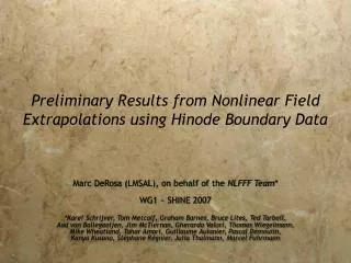
10. Hinode/XRT overlay - preflare fieldlines contained within a 320×320×128 pixel volume 2006.12.12_2030

11. Volume renderings of current pre-flare post-flare E/Epot=1.32 E/Epot=1.14

12. Volume renderings of current pre-flare post-flare E/Epot=1.32 E/Epot=1.14

13. Summary • NLFFF algorithms do not reach a consensus for this case. • Still, we can determine a best-matching model by comparing model fieldlines to observations in the EUV (from TRACE) and/or in x-rays (from Hinode/XRT). • In the best-matching model, free energy drops from 32% to 14% of potential energy, corresponding to a drop in free energy of 31032 erg, even as total field energy increased by ~1032 erg during this time. • Issue #1: EUV and x-ray coverage was not optimalfor this region, making it hard to determine best-fit model. (TRACE had only 285 binned 22, and x-ray images not the best for identifying loops.) • Issue #2: Lower boundary did not fully contain both flare ribbons. We are currently enlarging the lower boundary footprint and will repeat the analysis.