Approximating Bio-Pathways Dynamics
Approximating Bio-Pathways Dynamics. P.S. Thiagarajan School of Computing, National University of Singapore Joint Work with: Liu Bing, David Hsu. Bio-Pathways. Gene regulatory networks Metabolic pathways Signaling pathways. Signaling pathways.

Approximating Bio-Pathways Dynamics
E N D
Presentation Transcript
Approximating Bio-Pathways Dynamics P.S. Thiagarajan School of Computing, National University of Singapore Joint Work with: Liu Bing, David Hsu
Bio-Pathways Gene regulatory networks Metabolic pathways Signaling pathways
Signaling pathways • To sense external and internal environments of a cell: through a cascade of reactions. • A multitude of signaling pathways govern and coordinate the behavior of cells • Many disease processes arise from defects in signaling pathways:
The Basic Model • Signaling pathway • A network of bio-chemical reactions • Model: A system (network) of ODEs • One for each reaction • Study the ODE system to understand the dynamics of the signaling pathway • Many variations based on this basic model
We want to know……….. What is the concentration level of the protein p at time t (steady state)? Which initial conditions fit the data best? Sensitivity of reactions/parameters Effects of perturbations
Many Hurdles • Rate constant values are not known • must be estimated • Limited noisy data • High dimensional system • closed form solutions are impossible • Must resort to numerical simulations • a large number of simulations needed for answering each question
The Approximation Idea • Generate a “sufficiently” large number of “typical” trajectories. • View this ensemble as a representation of the dynamics. • This leads to a Markov chain model of the ensemble • Represent this Markov chain succinctly as a Bayesian network.
The Approximation Idea • Convert model analysis questions on ODEs to probabilistic inference problems on Bayesian networks. • good trade-off between accuracy and efficiency. • Pay one-time cost of constructing the Bayesian network. • Amortize this cost by performing multiple analysis tasks using the Bayesian network representation.
Discretize the value and time domains into intervals; A trajectory is a sequence of interval vectors. The Technique 3 1 3 2 0 2 0 0 1 0 0 0 ... ... ... ... 4 3 2 1 0 t0 t1
Main Idea The dynamics is the set of all possible trajectories State transition graph time 0 0 0 0 0 0 0 0 0 0 0 1 0 1 0 1 0 1 0 1 Prob(S11→S10)=0.8 1 0 1 0 1 0 1 0 1 0 1 1 1 1 1 1 1 1 1 1
Main Idea State transition graph Markov chain Pr(S[t+1]|S[t],S[t-1],...,S[1] )= Pr(S[t+1]|S[t]) time 0 0 0 0 0 0 0 0 0 0 0 1 0 1 0 1 0 1 0 1 Prob(S11→S10)=0.8 1 0 1 0 1 0 1 0 1 0 1 1 1 1 1 1 1 1 1 1
Main Idea A trajectory is a sequence of states The dynamics is the set of all possible trajectories State transition graph Markov chain time 0 0 0 0 0 0 0 0 0 0 0 1 0 1 0 1 0 1 0 1 1 0 1 0 1 0 1 0 1 0 1 1 1 1 1 1 1 1 1 1
Main Idea • A trajectory is a sequence of states • The dynamics is the set of all possible trajectories • State transition graph Markov chain • But the Markov chain will be huge! • 50 binary variables →250 states
Method Exploit the network structure to obtain a Bayesian network. Build BN structure (2 time-slice dynamic BN) directly. Fill up conditional probability tables S0 S3 S2 S1 E3 E2 E0 E1 ES3 ES0 ES2 ES1 P1 P0 P2 P3 ... ... ... ... ... ... ... ... P(S1=0|S0=0,E0=0,ES0=0)=0.2 P(S1=0|S0=1,E0=0,ES0=0)=0.4 ... ...
time X0 X1 X2 X3 X4 y0 y1 y2 y3 y4 Main Idea • Model analysis Bayesian inference • Given initial conditions, what is the probability distribution of Xi at any time T? • Use Inference! For instance, the FF algorithm.
Applications • Sensitivity analysis • Parameter estimation • Perturbation analysis • Parameter-free simulations. = ??
A Case Study • The EGF-NGF signaling pathway is important to understand how distinct signals dictate different cellular outcomes by activating the same signaling cascade Kholodenko 2007
A Larger Example ODE model 32 species 48 parameters 28 equations Features: Large size Feedback loops Brown et al. 2004
A Case Study • Approximate model Construction • Settings • 5 intervals, 1min time-step, 3 x 10⁶ samples • Runtime • 4 hours on a cluster of 10 PCs
BN-Simulation Results • Running time • Generating a stable nominal profile • 386.4 seconds • A single execution of FF inference • 0.29seconds • The total computation time will be sharply reduced when many such “queries” need to be answered by model analysis
Global Sensitivity Analysis • Running time • ODE based: 22 hours • BN based: 0.56 hours
This is all very well in practice but ... What about in theory? Degree of approximations Sampling technique Robustness Approximating the chemical master equation Probabilistic bounded model checking
Degree of approximations The flow is continuous and hence measurable Defines an idealized finite state Markov chain Infinite time horizon Discrete probability distributions but real-valued As number samples increases and the accuracy of the numerical integration improves, the quality of the approximation increases.
Sample size What is a good number? Why is the quality of approximation good? Dumb luck? Robustness? A framework for studying robustness?
Our Bayesian networks represent finite state Markov chains. compactly Formal verification techniques probabilistic bounded model checking Use SAT solvers?
Lab Members Faculty: David Hsu P.S. Thiagarajan Student s: Wang Junjie Geoffrey Koh Chin Yen Song Liu Bing Sucheendra Kumar Palaniappan Brandon Ooi Nick Sern Luo Weiwei
Collaborators Shazib Pervaiz Ding Jeak Ling Hanry Yu Marie-Veronique Clement