Download
1 / 75
760 likes | 988 Views
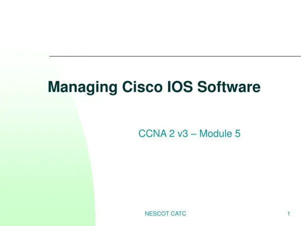
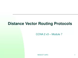
Routing in General Distance Vector Routing. Jean-Yves Le Boudec Fall 2009. Contents. 1. Routing in General 2. Distance vector Bellman-Ford How it is used in practice 3. Protocols that implement Distance Vector RIP RIP v2 IGRP 4. More about routing in general.

E N D
Routing in General Distance Vector Routing Jean-Yves Le BoudecFall 2009 1
Contents 1. Routing in General 2. Distance vector Bellman-Ford How it is used in practice 3. Protocols that implement Distance Vector RIP RIP v2 IGRP 4. More about routing in general 2
1. IntroductionWhy were routing protocols invented IP assumes routing tables are maintained at hosts and routers used by Packet Forwarding Routing = control method maintain routing tables automatically in routers At host routing tables are usually maintained by default rules plus ICMP redirect in old times: was done also by a routing protocol (RIP). Today, a host usually does not run any routing protocol Compare to: LANs connected by bridges operate at layer 2 like connectionless packet forwarders Q. How do they maintain routing information ? solution 3
Routing vs Packet Forwarding Packet Forwarding for every packet done in real time Routing computation of routing tables or data structures for unicast and multicast normally only between routers non-real time: latency up to 2 minutes uses dedicated protocols (RIP, OSPF, EIGRP (Cisco) for unicastand DVMRP, M-OSPF, PIM) ICMP-redirect may alter routing tables, but only in hosts 4
Interior Routing Routing methods are of two types Inside an administrative domain = Interior Routing Between domains = Exterior Routing Problem solved by a routing protocolWhat a routing protocol does find reachable destinations find best paths towards destinations best in the sense of some metric in this module, best means along shortest path, for some additive metric (number of hops, delay) 5
Metrics Distance vector and link state find paths that minimize a metric Static metric - does not depend on the network state; for example: number of hops link capacity and static delay cost Dynamic metric- depend on the network state link load current delay see end of section 6
Simple Routing MethodsHow routing protocols work static configuration for toy networks only flooding each packet duplicated on each outgoing link; loops prevented by packet id or other mechanism ; duplicate packets may be received at destination simple and robust no need for routing tables robust - tolerates link or router failures optimal in some sense the first packet has found the shortest path to the destination costly many duplicated packets – little useful traffic used as an ingredient by mobile ad-hoc routing methods (AODV, OLSR) source routing source writes route into packet header router reads next hop from packet header, moves pointer route discovered by flooding 7
Source Routing A B 2.2.4 SA DA RI data A B 2.2.4 A B 2.2.4 2 Q. What are the routes that can be used from A to B ? solution A route is described by a sequence of port numbers 1 1 IS 3 2 4 4 2 B A 1 IS 2 IS 3 3 1 IS 3 8
Route Discovery in Token Rings R3 R2 R6 B R5 A R1 R4 B2 B3 B6 B1 B5 B4 One “All Route Broadcast” packet is generated by A. This creates 5 different packets. 1. A-R1-B1-R2-B2-R3 2. A-R1-B1-R2-B3-R5-B6-R6 3. A-R1-B1-R2-B3-R5-B5-R4 4. A-R1-B4-R4-B5-R5-B3-R2-B2-R3 5. A-R1-B4-R4-B5-R5-B6-R6 2 of them reach B (numbers 2 and 5) route_1 = R1.B1.R2.B3.R5.B6.R6 route_2 = R1.B4.R4.B5.R5.B6.R6 9
In the 1980’s, the token was invented as a competitor to Ethernet. Bridging is in theory independent of whether we use token ring or ethrnet, however in practice token ring LANs used source routing bridges instead of spanning tree bridges.Source routing bridges work as illustrated on the figure: Bridges and token rings have numbers. Think of a token ring as functionally the same as an Ethernet collision domain Assume A has a packet to send to B (here A and B are MAC addresses, but this works equally well with IP addresses). A needs to find a description of a route to B. To this end, A floods the network with an “all-route-broadcast” packet. The packet is generated by A and sent over ring R1. This packet has a special destination address that means “all-route-broadcast”. All bridges listen to all rings that they are attached to (this is their job as forwarding devices). When they see a packet with destination address “all-route-broadcast”, they forward the packet to all other rings they are attached to, except if the packet has already visited this ring (the packet contains in its header the list of rings and bridges that it has already visited). For example, the packet created by A is seen by B1 [resp. B4] who forwards a copy on R2 [resp. R4]. B2 and B3 see the packet on R2 and forward it to R5 and R3. Etc. At some point in time, B4 sees a packet on R4 put by B5, which contains as list of visits: “A-R1-B1-R2-B3-R5-B5-R4” (packet number 3). This packet contains R1 in its list, therefore B4 does not forward it. This generates 5 packets in total (numbered 1 to 5 on the figure), 2 of them reach ring R6. When B sees any of them, it sends an acknowledgement to A. This ack is source routed, along the reverse route. A then receives two acks, each of them contains source route information that can be inverted by A. A now has two routes to B and can choose for example the shortest (in number of hops). DSR (Dynamic Source Routing) is a protocol for routing in ad-hoc networks that uses the same mechanism, but with IP addresses instead of MAC addresses. 10
Other Methods Distance vector (Bellman-Ford) routers only know their local state link metric and neighbor estimates interior routing protocols (RIP, IGRP) Link state knowledge of the global state topology database global optimization (Shortest Path First - Dijkstra) interior routing protocols (OSPF, PNNI (ATM)) Path vector no knowledge of the global state path: sequence of AS with attributes global optimization and policy routing exterior routing protocols (BGP) 11
2. Distance Vector Whatit does: Computes best paths to all destinations Fully distributed Using as only information the distances from self to all destinations How it works uses distributed Bellman-Ford – see next slides Note: individual link cost is setup by network management We first describe the centralized Bellman-Ford algorithm. 12
The Centralized Bellman-Ford Algorithm What: Given a directed graph with links costs A(i,j), computes the best path from i to j for any couple (i,j). We assume A(i, j) > 0 and A(i,j) = when i and j are not connected. How: Take for example j=1 and let p(i) be the cost of the best path from i to 1. Define pk(i) as the cost of the best path from i to 1 in at most k hops. Let p0(1) = 0, p0(i) = for i 1. (Bellman Ford, BF1) Theorem If the network is fully connected, the algorithm stops at the latest for k=n and then pk(i)=p(i) for all i The shortest path from i 1 to 1 is defined by pred(i) = Argminji [A(i,j) + p(j)]. Idea of Proof: pk(i) is the distance from i to 1 in at most k hops. Comment: recursion is equivalent to : pk(i) = min{ minji, j1 [A(i,j) + pk-1(j)] , A(i,1) } 13
Example Apply the theorem: write pk(i), pred(i) and draw the shortest paths to node 1.solution 3 6 1 1 2 1 3 3 1 5 4 1 14
Impact of Initial Conditions Example: Q. does the algorithm converge to the shortest path with initial condition as shown ?solution 3 k\i 1 2 3 4 5 0 0 0 0 0 0 1 2 3 4 k\i 1 2 3 4 5 0 0 6 1 1 0 1 2 3 4 6 1 1 2 1 3 3 1 5 4 1 15
Impact of Initial Condition Theorem The algorithm converges in a finite number of steps to the correct values for all initial conditions such that p0(1)=0 and for every node i that is connected to 1 If there is no path from i to 1, the algorithm lets pk(i) converge to 1 16
Proof We do the proof assuming all nodes are connected. Let pk be the vector pk[i], i=2,…. Let B be the mapping that transforms an array x[i]i=2…into the array Bx defined for i 1 by Bx[i]=min j i, j 1[A(i,j) + x(j)]Let b be the array defined for i 1 by b[i]= A(i,1)The algorithm can be rewritten in vector form as (1) pk = B pk-1 bwhere is the pointwise minimum Eq (1) is a min-plus linear equation and the operator B satisfies B(x y)= Bx By. Thus, Eq(1) can be solved using min-plus algebra into (2) pk = Bkp0 Bk-1b … Bb b Define the array e for i 1 by e[i]= . Let p0=e. Eq (2) becomes (3) pk = Bk-1b … Bb b. Now we have the Bellman Ford algorithm with classical initial conditions, thus, by Theorem 1: (4) for k n-1: Bk-1b … Bb b = qwhere q[i] is the distance from i to 1. We can rewrite Eq(2) for k n-1 as (5) pk = Bkp0 q Bkp0[i] can be written as A[i,i1]+ A[i1,i2]+ …+ A[ik-1,ik]+ p[ik] thus (6) Bkp0[i] k a, where a is the minimum of all A[i,j]. Thus Bkp0[i] tends to when k grows. Thus for k large enough, Bkp0 is larger than q and can be ignored in Eq(5). In other words, for k large enough : (6) pk = q 17
Distributed Bellman Ford BF1 can be used in a centralized algorithm to compute p(i) i.e. find the shortest path. However, this is not its main interest, because there is a better algorithm (Dijkstra) that can be used in a centralized method But: it can be distributed, as follows. Theorem: if the time to reliably send a message is bounded by T, the algo converges to the same result as the centralized version in at most nT time units (if the network is fully connected) • Distributed Bellman-Ford Algorithm v1, BFD1 • every node, say i, maintains an estimate q(i) of the distance p(i) to some fixed node 1; initial conditions are arbitrary but q(1)=0 at all steps • from time to time, i sends the new value q(i) to all its neighbours • when node i receives a value q(j0) from any neighbour j0, it sets q(j0) to the received value and updates q(i) by recomputingeq (1) q(i) := min j neighbour (A(i,j)+q(j)) • if eq (1) causes q(i) to be modified, pred(i) is set to a value of j that achieves the min 18
Distributed Bellman-Ford v1 A possible run of algorithm v1. The table shows the successive values of q(i) i 1 2 3 4 5 0 0 1 0 1 4 0 1 7 4 0 1 7 5 4 0 1 7 4 4 0 1 7 2 4 0 1 7 2 3 0 1 7 2 3 0 1 4 2 3 1 -> 2 2 -> 5 2 -> 3 5 -> 4 2 -> 4 1 -> 4 4 -> 5 5 -> 2 5 -> 3 link breaks 3 6 1 1 2 1 3 3 2 5 4 1 Q: give a possible scenario after link 4—5 breaks solution 19
Naive Distributed Bellman-Ford The previous distributed version requires a node to remember all previously received estimates q(j) for all neighbours, even if they are not the best ones In practice this is a problem if we need to compute the shortest paths to not just one destination, but to a large number. A naive distributed Bellman-Ford would be as v1 except we replace eq(1) by: Q. does this work ? why or why not ?solution Distributed Bellman-Ford Algorithm v1a, BFD1awhennode i receives new value q(j) fromnode j doeq (1a) q(i) := min { A(i,j) + q(j), q(i) } 20
Distributed Bellman-Ford, cont’d There is an alternative algorithm, that requires only to remember the best neighbour (pred(i)) • Distributed Bellman-Ford Algorithm, version 2 BFD2 • every node, say i, maintains an estimate q(i) of the distance p(i) to some fixed node 1; initial conditions are arbitrary but q(1)=0 at all steps • from time to time, i sends its value q(i) to all its neighbours • when node i receives a value q(j0) from any neighbour j0, it sets q(j0) to the received value and updates q(i) by recomputingeq (2)if j0 == pred(i) then q(i) := A(i,j0)+q(j0)else q(i) := min { A(i,j0) + q(j0), q(i) } • if eq (2) causes q(i) to be modified, pred(i) is set to j0 21
Distributed Bellman-Ford v2 Theorem: If the time to reliably send a message to all neighbours and perform local computations is bounded by T’, then the algorithm BFD2 converges to the correct values in at most m (T+T’) time units, where m is the number of steps of convergence of the centralized algorithm with same initial conditions Comment: The main difference with version 1 is that eq(2) replaces eq(1). Assume we use v2, and we start from a condition such that q(i) is indeed equal to the minimum given by eq (1) (which is what, intuitively, is true most of the time).When j is not equal to pred(i), both eq(1) and eq(2) have the same effect: the new value of q(i) is the same in both cases. In contrast, if j == pred(i), then eq (2) sets q(i) to the new value A(i,j)+q(j), whereas eq(1) sets it to minj neighbour (A(i,j)+q(j)).Eq(2) provides an upper bound on eq(1), in this case. It turns out that the algorithm still works, by the same mechanism that makes the algorithm work even when the initial conditions are arbitrary. Indeed, node i will send its new value to all remaining neighbours, who will in turn do an update and eventually, node i will receive values of q(j) that will correct the problem. In other words, if the new value of q(i) is too high (compared to what would be obtained with eq (1)), this is repaired in one round of exchanges with the neighbours. 22
Distributed Bellman-Ford v2 A possible run of algorithm v1: i 1 2 3 4 5 0 0 1 0 1 4 0 1 7 4 0 1 7 5 4 0 1 7 4 4 0 1 7 2 4 0 1 7 2 3 0 1 7 2 3 0 1 4 2 3 1 -> 2 2 -> 5 2 -> 3 5 -> 4 2 -> 4 1 -> 4 4 -> 5 5 -> 2 5 -> 3 link breaks 3 6 1 1 2 1 3 3 2 5 4 1 Q: give a possible scenario after link 4—5 breaks solution 23
How it is used in practice Node i computes shortest path and next hop for all network prefixes n that it heard of. Initially: D(i,n) = 0 if i directly connected to n and D(i,n) = + for any n that was never heard of. Node i receives from neighbour k latest values of D(k,n) for all n (this is the distance vector). Node i computes the best estimates according to algorithm BFD2 This converges if network is stable hello mechanism to reset computation after changes if neighbour k is no longer present, node i will no longer receive hello messages, and after a timeout, this has the same effect as if node i would receive the message from k: D(k,n)=1 for all n. Then algorithm BFD2 is run 1 D(1,n) c(i,1) c(i,k) D(k,n) i n k c(i,m) m D(m,n) 24
Example 1 net dist nxt net dist nxt n1 0 n1,A n4 0 n4,A n1 0 n1,B n2 0 n2,B A B n1 n4 n2 m2 n3 D C m3 m1 net dist nxt net dist nxt n3 0 n3,D n4 0 n4,D m3 0 m3,D n2 0 n2,C n3 0 n3,C m1 0 m1,C m2 0 m2,C A B D C 25
Example 1 net dist nxt net dist nxt n1 0 n1,A n4 0 n4,A n1 0 n1,B n2 0 n2,B n4 1 n1,A A B n1 n4 n2 m2 n3 D C m3 m1 net dist nxt n3 0 n3,D n4 0 n4,D m3 0 m3,D A B from A n1 0 n4 0 D C net dist nxt n2 0 n2,C n3 0 n3,C m1 0 m1,C m2 0 m2,C n4 1 n3,D m3 1 n3,D from D n3 0 n4 0 m3 0 26
Example 1 net dist nxt net dist nxt n1 0 n1,A n4 0 n4,A n1 0 n1,B n2 0 n2,B n3 1 n2,C n4 1 n1,A m1 1 n2,C m2 1 n2,C m3 2 n2,C A B n1 n4 n2 m2 n3 D C m3 m1 net dist nxt n3 0 n3,D n4 0 n4,D m3 0 m3,D B A from C n2 0 n3 0 m1 0 m2 0 n4 1 m3 1 D C net dist nxt n2 0 n2,C n3 0 n3,C m1 0 m1,C m2 0 m2,C n4 1 n3,D m3 1 n3,D 27
Example 1 - Final net dist nxt net dist nxt n1 0 n1,A n2 1 n1,B n3 1 n4,D n4 0 n4,A m1 2 n4,D m2 2 n4,D m3 1 n4,D n1 0 n1,B n2 0 n2,B n3 1 n2,C n4 1 n1,A m1 1 n2,C m2 1 n2,C m3 2 n2,C A B n1 n4 n2 m2 n3 D C m3 m1 net dist nxt net dist nxt n1 1 n4,A n2 1 n3,C n3 0 n3,D n4 0 n4,D m1 1 n3,C m2 1 n3,C m3 0 m3,D n1 1 n2,B n2 0 n2,C n3 0 n3,C m1 0 m1,C m2 0 m2,C n4 1 n3,D m3 1 n3,D A B D C 28
Example 1 - Failure net dist nxt n1 0 B n2 0 B n3 1 C n4 1 A m1 1 C m2 1 C m3 2 C A B n1 n4 n2 m2 n3 D C m3 m1 net dist nxt net dist nxt n1 1 A n2 1 C n3 0 D n4 0 D m1 1 C m2 1 C m3 0 D n1 1 B n2 0 C n3 0 C m1 0 C m2 0 C n4 1 D m3 1 D B We show only the router in the next hop field D C 29
Example 1 - Failure net dist nxt n1 0 B n2 0 B n3 1 C n4 1 A m1 1 C m2 1 C m3 2 C A B n1 n4 n2 m2 n3 D C m3 m1 net dist nxt net dist nxt n1 1 A n2 1 C n3 0 D n4 0 D m1 1 C m2 1 C m3 0 D n1 1 B n2 0 C n3 0 C m1 0 C m2 0 C n4 1 D m3 1 D B timeout D timeout C 30
Example 1 - Failure net dist nxt n1 0 B n2 0 B n3 1 C m1 1 C m2 1 C m3 2 C A B n1 n4 n2 m2 n3 D C m3 m1 net dist nxt net dist nxt n1 2 C n2 1 C n3 0 D n4 0 D m1 1 C m2 1 C m3 0 D n1 1 B n2 0 C n3 0 C m1 0 C m2 0 C n4 1 D m3 1 D B D From C: n1 1 B n2 0 C n3 0 C m1 0 C m2 0 C n4 1 D m3 1 D C 31
Example 1 - After Failure net dist nxt n1 0 B n2 0 B n3 1 C n4 2 C m1 1 C m2 1 C m3 2 C A B n1 n4 n2 m2 n3 D C m3 m1 net dist nxt net dist nxt n1 2 C n2 1 C n3 0 D n4 0 D m1 1 C m2 1 C m3 0 D n1 1 B n2 0 C n3 0 C m1 0 C m2 0 C n4 1 D m3 1 D B D C 32
Example 1: conclusions Example 1 illustrates how Bellman Ford is mapped to the network concepts how topology changes are taken into account most recent announcement replaces previous ones non refreshed announcements become obsolete how distance vector carries reachability information 33
Example 2 A B l1 l2 C l3 l4 l5 l6 D E To simplify, we identify destination with router Assume algorithm has converged A B dest link cost dest link cost A local 0 B l1 1 D l3 1 C l1 2 E l1 2 B local 0 A l1 1 C l2 1 E l4 1 D l1 2 C cost =1 dest link cost cost =1 C local 0 A l2 2 B l2 1 D l2 3 E l2 2 cost =1 cost =5 D E cost =1 dest link cost dest link cost D local 0 A l3 1 B l3 2 C l3 3 E l6 1 E local 0 A l4 2 B l4 1 D l6 1 C l4 2 34
Example 2 • we now show only table entries: to C • link 2 fails • B updates its table C l1 2 C l2 A B l1 C l3 l4 C local 0 l5 l6 D E C l3 3 C l4 2 35
Example 2: Link failure • Just before B updates its table, A broadcasts its table with cost 2 to C • B updates C l1 2 C l1 3 from A: C l1 2 A B l1 C l3 l4 C local 0 l5 l6 D E C l3 3 C l4 2 36
Example 2: Link failure • B sends update to A and E • A and E update C l1 4 C l1 3 from B: C l1 3 A B l1 C l3 l4 C local 0 l5 l6 D E from B: C l1 3 C l3 3 C l4 4 37
Example 2: Link failure • C sends update • it is ignored by E because it it less good C l1 4 C l1 3 A B l1 C l3 l4 C local 0 l5 l6 D E from C: C local 0 C l3 3 C l4 4 38
Example 2: Link failure • A broadcasts its table with cost 4 to C • B updates … we have a loop between A and C • cost is increase by 2 at every iteration C l1 4 C l1 5 from A: C l1 4 A B l1 C l3 l4 C local 0 l5 l6 D E C l3 3 C l4 4 39
Example 2: Link failure • E now accepts announcement from C C l1 6 C l1 7 A B l1 C l3 l4 C local 0 l5 l6 D E from C: C local 0 C l3 7 C l5 5 40
Example 2: Link failure • E sends announcements to D and B • B and D send announcements to A • the algorithm has converged – stable state C l1 7 C l4 6 from B: C l4 6 from E: C l5 5 A B l1 C l3 l4 C local 0 l5 l6 D E from E: C l5 5 C l6 6 C l5 5 41
Conclusions from Example 2 the algorithm converges after modification of the topology, but the convergence may be very slow bounce effect Q: during convergence time, how are routing tables ?solution 42
Example 3 Assume now all link costs are equal to 1 Links l1 and l6 fail D detects failure and sets costs to 1 A B dest link cost dest link cost A local 0 B l3 3 D l3 1 C l3 3 E l3 2 B local 0 A l4 3 C l2 1 E l4 1 D l4 2 C dest link cost A B C local 0 A l5 3 B l2 1 D l5 2 E l5 1 l2 C l3 l4 l5 D E D E dest link cost dest link cost D local 0 A l3 1 B l3 C l6 E l6 E local 0 A l6 2 B l4 1 D l6 1 C l5 1 43
Example 3 A A A dest link cost dest link cost dest link cost A local 0 B l3 3 D l3 1 C l3 3 E l3 2 A local 0 B l3 5 D l3 1 C l3 5 E l3 4 A local 0 B l3 3 D l3 1 C l3 3 E l3 2 from A: dest cost A 0 B,C 3 D 1 E 2 from B: dest cost A 1 B,C 4 D 0 E 3 from A: dest cost A 0 B,C 5 D 1 E 3 A A A l3 l3 l3 D D D D D D dest link cost dest link cost dest link cost D local 0 A l3 1 B l3 4 C l3 4 E l3 3 D local 0 A l3 1 B l3 4 C l3 4 E l3 3 D local 0 A l3 1 B l3 6 C l3 6 E l3 5 44
Conclusion from Example 3 The costs to C, B, E grow unbounded “Count to Infinity” the true costs are infinite Convergence to a stable state if we set = large number e.g. RIP: = 16 “Split Horizon” a heuristic to prevent this if A routes packets to X via B, it does not announce this route to B 45
Example 3: with Split Horizon A B dest link cost dest link cost A local 0 B l3 3 D l3 1 C l3 3 E l3 2 B local 0 A l4 3 C l2 1 E l4 1 D l4 2 C dest link cost A B C local 0 A l5 3 B l2 1 D l5 2 E l5 1 l2 C l3 l4 l5 D E D E dest link cost dest link cost D local 0 A l3 1 B l3 C l6 E l6 E local 0 A l6 2 B l4 1 D l6 1 C l5 1 46
Example 3: with Split Horizon A dest link cost A local 0 B l3 3 D l3 1 C l3 3 E l3 2 from A: dest cost A 0 A l3 D D dest link cost D local 0 A l3 1 B l3 C l6 E l6 47
Split horizon A • Split horizon cuts the process of counting to infinity dest link cost A local 0 B l3 D l3 1 C l3 E l3 from D: dest cost D 0 B,C,E A l3 D D dest link cost D local 0 A l3 1 B l3 C l6 E l6 48
Split horizon may fail B dest link cost from E: dest cost A B 1 C 1 D B local 0 A l4 C l2 1 E l4 1 D l4 C dest link cost B C local 0 A l5 3 B l2 1 D l5 2 E l5 1 l2 C l4 l5 E E dest link cost E local 0 A l6 B l4 1 D l6 C l5 1 49
Split horizon may fail B from C: dest cost A 3 D 2 E 1 dest link cost B local 0 A l24 C l2 1 E l4 1 D l2 3 C dest link cost B C local 0 A l5 3 B l2 1 D l5 2 E l5 1 l2 C l4 l5 E E dest link cost from C: dest cost B 1 E local 0 A l6 B l4 1 D l6 C l5 1 50