Chapter 7-2 Sensitivity Analysis

1. Chapter 7-2 Sensitivity Analysis by Dr. Peitsang Wu Department of Industrial Engineering and Management I-Shou University

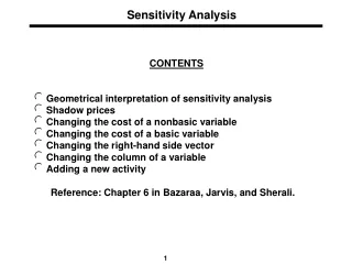
2. Sensitivity Analysis • Change in the right hand side (bi). • Change in the cost coefficient . • Coefficient of the non-basic variables (cN). • Coefficient of the basic variables (cB). • Change in A. • Adding a new variable. • Removing a variable. • Adding a constraint. • Removing a constraint.

3. Change in b • As long as the r.h.s. of each constraint in the optimal tableau remains non-negative, the current basis remains feasible and optimal. • If at least on r.h.s. in the optimal tableau becomes negative, the current basis is no longer feasible and therefore no longer optimal.

4. Change in b • In order to declare that B is an optimal basis , we have to check two conditions . (1) rT= B-1N- is non-negative (true , no b inside ) (2) B.F.S. is feasible (i.e. ) (need to check) Let Our new L.P model Max z=cTx s.t. Ax=b+ b must

5. Example 7.2 original model new model

6. Example 7.2(Cont.) • Final tableau for original problem

7. Example 7.2(Cont.) And = B-1(b+b)= which is not feasible!

8. Example 7.2(Cont.) Here B-1=yT • Use the dual simplex method to find another B.F.S. satisfies and gets (x1,x2,x3,x4,x5)=(0,9,4,6,0) , and z = 45 Discuss later!

9. Change in b • What’s the upper and lower bound for changing bi？ • Recall • Example:

10. Example 7.3 solve for ? consider only

11. Example 7.3(Cont.) and the basis is remain feasible called the allowable range to stay feasible, and = B-1(b+  b) =36+ B-1  b=36+ =36+ so

12. Change in cN • change in cN will not influence B, B-1,b, and the basic variables are still unchanged. • The only change is the coefficient of that non basic variable. • If ( for the new coefficient of the non-basic variable )then the optimal condition is unchanged. • If then the current B.F.S is not optimal anymore. We have to repeat simplex iteration to get new optimal solution.

13. Change in cN Question：What is the range of such that, the optimal tableau remains optimal？ i.e. = B-1N – for all for some q with , = B-1Nq- Let = cq+ = B-1Nq– = rq (the allowable range to stay optimal)

14. Example 7.4

15. Change in cB • The change in cB will not change B, B-1, or b and the basic variables are still unchanged. • However, will change, this may change more than one coefficient in row 0. • We need to re-compute row 0, if each variable in row 0, the current basic variables are still optimal. Otherwise, re-compute the simplex tableau.

16. Change in cB • Question：What’s the range of such that the optimal tableau remains optimal？ i.e. = B-1Nq – for all for some = B-1Nq–

17. Example 7.5 Let r4= B-1N4 –c4

18. Example 7.5(Cont.) r5= B-1N5- c5

19. Example 7.5(Cont.) the allowable range to stay optimal: z =36+ =36+

20. Change in A (a) adding a new variable xn+1 Max s.t. We can set xn+1=0 then becomes a B.F.S. for the new L.P. We only need to check rn+1= or < 0 if rn+1> 0 we do not need to do anything, the current B.F.S is optimal. Otherwise, enter xn+1as the basic variable, re-compute simplex tableau.

21. Change in A (b) removing a variable xk • If xk*=0, then the current optimal solution x* remain optimal otherwise (i.e. xk*＞0, xk* is a basic variable), we have to work out a new solution.

22. Change in A • We can remove xk by solving the phase I problem： Min xk s.t. Ax=bx 0 (use x* be the initial feasible solution) If the optimal solution , then removing xk will cause the original problem infeasible. Otherwise, if take the optimal tableau of phase I problem as the initial tableau of phase II problem.

23. Change in A (c) Adding a constraint let new constraint (L.P) Max cTx s.t. Ax=b x* new constraint (x* infeasible) (x* feasible) new constraint

24. Adding a constraint • The new constraint may cut the original feasible region to be smaller. • If x* remains feasible, then of course it remains optimal. • If x* was excluded from the new feasible region, we do not have a B.F.S to start, also B is not longer a basis in the new problem.

25. How to solve Max S.t. BxB+ NxN= b (am+1,B)TxB +(am+1,N)TxN + xn+1=bm+1 xB , xN, xn+1 Where am+1,B, am+1,N are the sub rows of am+1 corresponding to xB and xN.

26. How to solve is a basic solution to the new problem (not necessary feasible).

27. Adding a constraint • Lemma 1 Let B be an optimal basis to the original L.P. problem, If define above, is non negative, then it is an optimal solution to the new L.P. problem with additional constraint. • Note: If is not non-negative, then the primal feasibility condition is violated by at lease one primal variable. In this case use the dual simplex algorithm starting a dual B.F.S. where

28. Adding a constraint • Consider the following problem:

29. Adding a constraint • The original optimal tableau is:

30. Adding a constraint

31. Adding a constraint

32. Change in A (d) removing a constraint • If the constraint , say is non binding (i.e. ) then it can be removed without affecting the optimality of the current optimal solution. (check yk = 0 then k-th constraint non binding by the complementary slackness) • On the other hand, resolve the new L.P. problem form the beginning.

33. Dual Simplex Method • Primal feasible: if the complementary primal basic feasible solution is feasible. • Dual feasible: if the complementary dual basic solution is feasible. • Each complementary basic solution is optimal if it is both primal feasible and dual feasible. • The dual simplex method can be thought of as the mirror of the simplex method.

34. Why Dual Simplex Method? • It may be easier to begin with a dual simplex method when too many artificial variables are introduced. • Use for the sensitivity analysis when minor changes force the primal feasible solution infeasible, i.e., the optimal feasible basic solution Is no longer primal feasible but still satisfies the optimally test . • Use for solving huge linear programming problem.

35. Dual Simplex Method • The coefficients in row 0 must be non-negative (optimal in the simplex tableau, and the basic solution is dual feasible). • The basic solutions will be infeasible only because some of the variables are negative. • The method continues to decrease the value of the objective function, always retaining nonnegative coefficients in row 0 an, until all the variables are nonnegative. • Such a basic solution is feasible and is optimal.

36. Procedure of Dual Simplex Method • Initialization: • Converting any functional constraints in  form to  form (by multiplying through both sides by –1). • Introduce slack variables as needed. • Find a basic solution such that the coefficients in row 0 are zero for basic variables and nonnegative for nonbasic variables.

37. Procedure of Dual Simplex Method • Feasibility Test: • Check to see whether all the basic variables are nonnegative. • If they are, then the current solution is feasible, and therefore optimal. STOP. • Otherwise, go to an iteration.

38. Procedure of Dual Simplex Method • Iteration: • Step 1: Determine the leaving basic variable by selecting the negative basic variable with the largest absolute value. • Step 2: Determine the entering basic variable by selecting the nonbasic variable with negative coefficient in that equation whose ratio of row 0 to the coefficient in that equation is the smallest absolute value. • Step 3: Determine the new basic variable by Gaussian Elimination.

39. Example

40. Convert to Dual Problem

41. Example

42. Example

43. Example