Download
1 / 38
390 likes | 761 Views
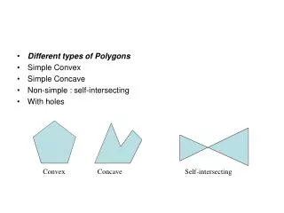
Different types of Polygons Simple Convex Simple Concave Non-simple : self-intersecting With holes. Convex. Concave. Self-intersecting. Polygon Scan Conversion. Scan Conversion = Fill How to tell inside from outside Convex easy Nonsimple difficult Odd even test Count edge crossings.

E N D
Different types of Polygons • Simple Convex • Simple Concave • Non-simple : self-intersecting • With holes Convex Concave Self-intersecting
Polygon Scan Conversion • Scan Conversion = Fill • How to tell inside from outside • Convex easy • Nonsimple difficult • Odd even test • Count edge crossings odd-even fill
Winding Number • Count clockwise crossings as positive and counterclockwise crossings as negative • Alternate definition of inside: inside if winding number 0 winding number = 1 winding number = 2
Filling in the Frame Buffer • Fill at end of pipeline • Convex Polygons only • Nonconvex polygons assumed to have been tessellated • Shades (colors) have been computed for vertices (Gouraud shading) • March across scan lines interpolating shades • Incremental work small
Using Interpolation C1 C2 C3 specified by glColor or by vertex shading C4 determined by interpolating between C1 and C2 C5 determined by interpolating between C2 and C3 interpolate between C4 and C5 along span C1 C4 C2 scan line C5 span C3
Interior pixels along a scan line passing through a polygon area Scan Line Polygon Fill • Determine overlap Intervals for scan lines that cross that area. • Requires determining intersection positions of the edges of the polygon with the scan lines • Fill colors are applied to each section of the scanline that lies within the interior of the region. • Interior regions determined as in odd-even test 10 13 16 19
10 13 16 19 • In the given example, four pixel intersections are at x=10, x=13, x=16 and x=19 • These intersection points are then sorted from left to right , and the corresponding frame buffer positions between each intersection pair are set to specified color • 10 to 13, and 16 to 19
Scan Line Polygon Fill • Some scan line intersections at polygon vertices require special handling: • A scan line passing through a vertex intersects two polygon edges at that position
Scan Line y’ 1 1 2 Scan Line y 1 1 1 2 Intersection points along the scan lines that intersect polygon vertices. Scan line y’ generates an even number of intersections that can be paired to identify correctly the interior pixel spans. To identify the interior pixels for scan line y, we must count the vertex intersection as only one point.
Scan Line Polygon Fill • The topological difference between scan Line y and scan Line y’ • For scan line y, the two edges sharing an intersection vertex are on opposite sides of the scan line. • Count this vertex as one intersection point • For scan line y’, the two intersecting edges are both above the scan line
Scan Line Polygon Fill • We can distinguish these cases by tracing around the polygon boundary either in clockwise or counterclockwise order and observing the relative changes in vertex y coordinates as we move from one edge to the next. • Let (y1, y2) and (y2, y3) be the endpoint y values of two consecutive edges. If y1, y2, y3 monotonically increase or decrease, we need to count the middle vertex as a single intersection point for any scan line passing through that vertex.
Scan Line Polygon Fill • One method for implementing the adjustment to the vertex intersection count is to shorten some polygon edges to split those vertices that should be counted as one intersection • When the end point y coordinates of the two edges are increasing , the y value of the upper endpoint for the current edge is decreased by 1 • When the endpoint y values are monotonically decreasing, we decrease the y coordinate of the upper endpoint of the edge following the current edge
Scan Line Polygon Fill Algorithm (a) (b) Adjusting endpoint values for a polygon, as we process edges in order around the polygon perimeter. The edge currently being processed is indicated as a solid like. In (a), the y coordinate of the upper endpoint of the current edge id decreased by 1. In (b), the y coordinate of the upper end point of the next edge is decreased by 1
The scan conversion algorithm works as follows • Intersect each scanline with all edges • Sort intersections in x • Calculate parity of intersections to determine in/out • Fill the “in” pixels • Special cases to be handled: • Horizontal edges should be excluded • Vertices lying on scanlines handled by shortening of edges, • Coherence between scanlines tells us that • Edges that intersect scanline y are likely to intersect y + 1 • X changes predictably from scanline y to y + 1 (Incremental Calculation Possible)
The slope of the edge is constant from one scan line to the next: • let m denote the slope of the edge. • Each successive x is computed by adding the inverse of the slope and rounding to the nearest integer
Integer operations • Recall that slope is the ratio of two integers: • So, incremental calculation of x can be expressed as
Integer operations • How to compute x intercepts incrementally using integer operations: • Initialize a counter to 0 • Increment counter by Dx each time we move up to a new scan line. • If counter becomes greater or equal to Dy, increment the current x intersection value by 1 and decrease the counter by Dy
Example: m=7/3 • Initial scanline counter = 0 • Next scanlines • Counter =3 • Counter =6 • Counter =9 • increment x intercept by • Reset counter to 9-7 = 2
Line with slope 7/3 yk xk
0 4 1 5 decrement decrement 2 6 3 0 decrement y0 counter x0
Above scheme truncates integers. • How do we round to nearest integer? • We need to compare the counter to Dy/2. • Can be done by integer arithmetic by incrementing counter by 2Dx at each step and comparing with Dy • When the counetr is greater than or equal to Dy, increase x value by 1 and decrement the counter by 2Dy
Example: m=7/3 • Initial scanline counter = 0 • Next scanlines • Counter =6 • Counter =12 • increment x intercept by • Reset counter to 12-(2*7) = -2
0 -6 2 -4 decrement decrement 4 -2 6 0 decrement y0 counter x0
Sorted Edge Table (SET) • In SET, there is an entry for each scanline. • Traverse edges of the polygon to construct a Sorted Edge Table (SET) • Eliminate horizontal edges • Add edge to linked-list for the scan line corresponding to the y_lower vertex. Shorten edges if necessary to resolve the vertex-intersection problem. • For each edge entry, store the following: • y_upper: the largest y value on that edge (last scanline to consider) • x_lower: the x intercept at that scanline (initial x value) • 1/m: for incrementing x • For each scan line the edges are sorted from left to right (based on x)
B C E C’ D A 1 0
Active Edge List (AEL) • Construct Active Edge List during scan conversion. AEL is a linked list of active edges on the current scanline, y. The active edges are kept sorted by x • The active edge list contains all the edges crossed by that scan line. • As we move up, update the active edge list using the sorted edge table if necessary.
Algorithm • Set y to the smallest y coordinate that has an entry in the SET; i.e, y for the first nonempty bucket. • Initialize the AEL to be empty. • For each scanline y repeat: • 3.1 Copy from SET bucket y to the AEL those edges whose y_min = y (entering edges). • 3.2 The sort the AEL on x is easier because SET is presorted. • 3.3 Fill in desired pixel values on scanline y by using pairs of x coordinates from AEL. • 3.5 Remove from the AEL those entries for which y = y_max (edges not involved in the next scanline.) • 3.4 Increment y by 1 (to the coordinate of the next scanline). • 3.5 For each nonvertical edge remaining in the AEL, update x for the new y.
Flood Fill Algorithm • These algorithms assume that at least one pixel interior to a polygon or region is known -assume that the boundary is defined by Bresenham’s
Flood Fill • Fill can be done recursively if we know a seed point (x,y) located inside (WHITE) • Scan convert edges into buffer in edge/inside color (BLACK) flood_fill(int x, int y) { if(read_pixel(x,y)= = WHITE) { write_pixel(x,y,BLACK); flood_fill(x-1, y); flood_fill(x+1, y); flood_fill(x, y+1); flood_fill(x, y-1); } }
Depth or Z-Buffer • For each pixel, we store COLOR (color buffer) and DEPTH (depth buffer). • Algorithm: Initialize all elements of buffer COLOR(row, col) to background color, and DEPTH(row, col) to maximum-depth; FOR EACH polygon: Rasterize polygon to frame; FOR EACH pixel center (x, y) that is covered: IF polygon depth at (x, y) < DEPTH(x, y) THEN COLOR(x, y) = polygon color at (x, y) AND DEPTH(x, y) = polygon depth at (x, y)
Depth Buffer Operation Frame Depth Initialize (“New Frame”)
Depth Buffer Operation – First Polygon Frame Depth 24 26 27 28 29 30 Pink Triangle -- depths computed at pixel centers
Depth Buffer Operation -- First Polygon Frame Depth 24 26 27 28 29 30 Pink Triangle -- pixel values assigned
Depth Buffer Operation – Second Polygon Frame Depth 10 9 24 9 8 26 8 7 28 7 6 Green Rectangle -- depths computed at pixel centers
Depth Buffer Operation – Second Polygon Frame Depth 10 9 24 9 8 26 8 7 28 7 6 Green Rectangle -- pixel values assigned: NOTE REPLACEMENTS!
Depth Buffer Operation – Third Polygon 68 not stored Frame Depth 10 9 72 24 9 8 75 26 8 7 71 not stored 7 28 6 Blue Pentagon -- depths computed at pixel centers
Depth Buffer Operation – Third Polygon Frame Depth 10 9 72 24 9 8 75 26 8 7 7 28 6 Blue Pentagon -- pixel values assigned: NOTE ‘GOES BEHIND’!
screen scan-line