Download
1 / 37
370 likes | 443 Views
Learn about the advantages and limitations of grating spectrometers for environmental research. Explore innovative imaging techniques and trace gas detection methods using different camera schemes. Discover active plume imaging techniques and understand the concept of Gas Correlation Spectroscopy.

E N D
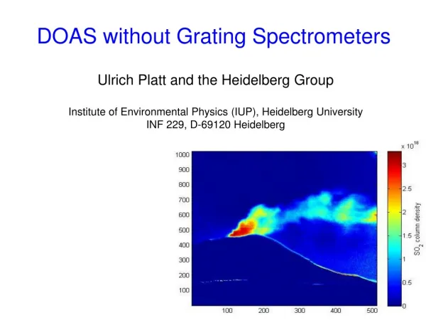
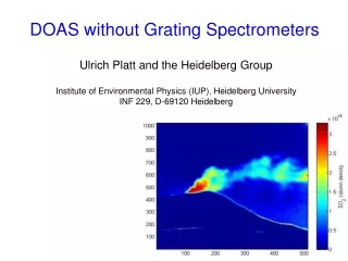
DOAS without Grating Spectrometers • Ulrich Platt and the Heidelberg Group • Institute of Environmental Physics (IUP), Heidelberg University • INF 229, D-69120 Heidelberg
Entrance Slit Grating Focal Plane The DOAS Workhorse: Grating Spectrometers Typical: Czerny Turner arrangement Advantages: Proven, successfull, reliable, known properties (?) Reasons not to use grating spectrometers: • Limited spectral range • Overlapping orders • Rather low light throughput and high straylight levels • Difficult to use in imaging applications
B) Column at a time “Push-Broom Imaging" • A) Pixel at a time “Whiskbroom Imaging" • C) Frame at a time (Full Frame) • A • B • C Dispersive spectroscopy possible with „Imaging spectrometers“ Usually dispersive spectroscopy • non-dispersive spectroscopy • Imaging FTIR I) 2D - Image Scanning Schemes in a 4-dimensional World Present technology only allows to use 3 Dim., 2 Space + Time = Wavelength FP = Focal Plane
The Importance of the “Photon Budget” (100x100 pixels) F3.21016 photons/(s m2 sr nm) • We need all the light we can get SO2: 20 ppmm
„Differential“ Absorption Spectroscopy(may not really be DOAS) Example: The „Trace Gas Camera“ (frequently used as „SO2 Camera“
Four Different Trace Gas Camera Schemes • Wavelength-Selective Element: • a) two narrow band filters alternatingly being brought into the beam SO2 - Camera • b) a Fabry-Perot interfero-meter with adjustable transmission wavelength FP - Camera • c) a narrow-band inter-ference filter, which can be rotated Filter Camera • d) a cell (cuvette) containing the gas to be measured, periodically introduced into the light beam Gas Correlation Camera • Alternative Position of WSE
a) Filter Camera (SO2-Camera): True 2-Dimensional Observation A B • Calculate SO2 column-density from ratio of intensities seen through filter A (IA) and Filter B (IB)and some normalisation and correction … • UV: Mori & Burton 2006, Bluth et al. 2007 ff. • IR: e.g. Prata and Bernardo 2009
b) Fabry-Perot – Interferometer-Based SO2-Spectrometer • SO2-Camera See next presentation by Jonas Kuhn • Fabry-PerotSpectrometerSetting APlate Dist. LA • Fabry-PerotSpectrometerSetting BPlate Dist. LB • Kuhn J., Bobrowski N., Lübcke P., Vogel L., Platt U. (2014), A Fabry-Perot interferometer based camera for two-dimensional mapping of SO2 distributions, Atmos. Meas. Tech. 7, 3705–3714.
c) The SO2-Camera, Rotating Filter - Design - non dispersive • 0o • 35o • Problems: 1) Wavelengths are not the same throughout the image2) image as a whole shifts position as the filter is tilted, Problems can be solved by applying image processing techniques or by adding a “guiding LED” (Benton et al. 2013) • Transmitted intensity of an interference filter: Incidence angles 0°(rightmost curve) to 35°(left) in steps of 1°. (Nominal central wavelength (i.e. at 0°incidence angle) is 458nm, however, any central wavelength (e.g. 300 nm) is possible. (from Zielcke et al. 2013)
I0 I0+Plume I0 I0+Cell I0+Cell+Plume d) Gas Correlation Spectroscopy • Idea: Ratio images recorded with- and without cell with gas to be measured in place • Gas cell attenuates less, if gas is present in the atmosphere! Use in industrial monitoring and on satellites e.g. Ward and Zwick 1975,Sandsten et al. 1996, 2004
SO2 • BrO e) Imaging DOAS (I-DOAS), Whisk-Broom • Example: Etna, May 10, 2005, Louban et al. 2006:
f) Passive IR-Imaging (Thermal Emission) • Emission spectrum instead of absorption, i.e. I() looks like () • Planck function • 1) Michelson interferometer + whisk-broom scanner 2-D images (Svanberg 2002, Rusch and Harig 2010, Stremme et al. 2012). • 2) Michelson interferometers + push-broom scanner (i.e. moving platform) 2-D images (Wright et al. 2013) • 3) IR-cameras with two or more filters (similar way to SO2 camera) (e.g. Prata and Bernardo 2009) for SO2 retrieval and ash detection (Prata and Bernardo 2014) • 4) Gas-correlation spectroscopy in the IR for imaging of ammonia and ethylene (e.g. Sandsten et al. 1996, 2004). • 5) Recent development: 2-D Michelson interferometers where instead of a single detector an array of detectors is used. Effectively each pixel can be thought of having its own interferometer. (e.g. GLORIA, Friedl-Vallon et al. 2006, using a 256 x 256 elements Mercury Cadmium Telluride focal plane array cooled to 60 K. (spectral coverage 7.1 m to 12.8 m) • (4)
Active: Artificial Light Source • LIDAR II) Active Plume Imaging Techniques
LASER • Detector • Trace Gas or • Aerosol - Cloud • R Classic (Mono-Static) LIDAR vs. Bi-Static LIDAR • 1) There is no need for a pulsed light source, in fact light emitting diodes in combination with suitable optics can be used. • 2) No need for a high time-resolution detector, radiation is received by a telescope – spectrometer combination, see customary active DOAS approach (e.g. Platt and Stutz. 2008). • 3) Further possibility: non-dispersive approach with two UV-LEDs emitting at "on absorption" and "off absorption" wavelengths. Example: LEDs emit in the wavelength ranges of filters A, B of a SO2-camera non-dispersive approach. • Classic Lidar
Bi-Static LIDAR – DOAS (BISL – DOAS) • Interesting: • Extent of overlap-region varies R2 • Compensates 1/R2 • 20 cm dia. Telescope + Detector (Spectrometer) • 6 cm dia. Lens + UV-LED
Radiative power budget of a Bi-Static LED-LIDAR System, R=1000m • AAt a photon energy of EP = hc/ 6.8510‑19 J at = 290nm (c = speed of light, h = Planck's constant) • 24 photoelectrons/(pixel s) • For just one LED! (could also use 10 LEDs) • 1% O.D. (SO2: 14 ppmm) detectable after 400s integration time SO2-camera 2-wavelength approach (2 LEDs with different wavelengths): 4s
Bi-Static LED-LIDAR System - Further Possible Geometries • Determination of the Integral cross section of the plume, note that no "light dilution" can occur • Geometry for probing the 2-D gas distribution in the plume
Collimating Lens CameraLens Index of refraction n() FocalPlane Entrance Slit Prism f2 f1 O 3 2 A B 4 1 III) Replace Grating Spectrometers by Prism Spectrometers Dispersion of a Prism: Total deviation between incoming and outgoing beam: = 1 - 2 - 3 + 4. In triangle OAB: = 2 + 3 = 1 + 4 - for small angles we have: = (n-n0) 0.5 (since n0 1.0, n 1.5) Rays of polychromatic light will be refracted in different directions with the total angular deviation: dn/d: change of the refractive index with wavelength, the dispersion, which for most glass types is of the order of 10-4 – 10-3 nm-1.
dn/d810-4/nm dn/d210-4/nm dn/d10-3/nm Dispersion of Various Types of Glasses
Dispersion of some Types of Glass 25x25mm: ca. 80€ BK7: n = SQRT( 1 + 1.03961212*x**2/(x**2-0.00600069867) + 0.231792344*x**2/(x**2-0.0200179144) + 1.01046945*x**2/(x**2-103.560653) ) x = wavelength in micrometers
Collimating Lens CameraLens FocalPlane Entrance Slit Prism f2=100mm f1=100mm A Sample Prism Spectrometer (1) Assuming prism with apex angle = 60o (1.047 radian) and dn/d 610-4 we have: e.g. Dense Flint at 400nm Need a detector with 5 m pixel size and 30 m entrance slit width in order to obtain a spectral resolution of 0.5nm (in the blue spectral region)
Collimating Lens CameraLens Entrance Slit Prism 1 Prism 2 FocalPlane f1=100mm f2=100mm Sample Prism Spectrometer (2) Entrance slit width = 30m 17nm/mm * 0.03 mm 0.51 nm Resolution Notes: 1) Slit could be very high (long) if e.g. a detector with 20 x 20 mm size is used 2) Angle of incidence on refracting surface is about: /2 + /2 23o + 30o 53oFresnel reflection @ 53o is about 6-7% 90% efficiency! 3) Dispersion curve is highly non-linear Needs to be corrected (linearisation before evaluation should be no problem) Allows very large spectral range with high resolution in the UV low resolution in the visible spectral range. 4) No overlapping orders 5) Resolution could be improved by using several prisms (e.g. two quartz prisms would give 0.5 nm resolution at 300 nm)
Summary • Imaging spectroscopy is an emerging field allowing new applications • In many cases limited spectral information is sufficient • Several new techniques are being introduced: - Imaging FTIR systems - Fabry-Perot Cameras • Techniques, which are already proven in other areas of research can be adapted: - Gas Correlation Spectroscopy - Filter Cameras • Further new techniques have been proposed or are in promising states of development: - LED-LIDAR - Wavelength-sensitive Pixel Detectors - Quantum entanglement imaging (Zeilinger et al. 2014) • Prism spectrometers may offer advantages for „classical“ DOAS applications
Many Different Geometries are Possible • Example: NO2-measurements using blue (450nm) LEDs • Array of 100 3W blue LEDs • From: Stephan Flock, Diploma Thesis, U. Heidelberg 2012
Minimum Detectable Mixing Ratio (ppb) • Light-path 1360m • Relative intensity • Light-path 750 m Fraction of Received Radiation Intensity and Detection Limit (for NO2 at 440 nm) • 1 • Light-path530 m • From: Stephan Flock, Diploma Thesis, U. Heidelberg 2012 • ca. 10 ppb NO2 detectable at 3 hour measurement time (Flock 2012) • 100 • Receiving Telescope elevation angle (degrees) • 30° Light source elevation angle, • Distance Teleskope – Light Source: 26.85 m • Light source: 300 W (input power) LED-array (about 60 W radiation intensity)
SO2-Camera • Fabry-PerotSpectrometerPos. APlate Dist. LA • Fabry-PerotSpectrometerPos. BPlate Dist. LB Fabry-Perot – Interferometer-Based SO2-Spectrometer • Kuhn J., Bobrowski N., Lübcke P., Vogel L., Platt U. (2014), A Fabry-Perot interferometer based camera for two-dimensional mapping of SO2 distributions, Atmos. Meas. Tech. Discuss. 7, 5117–5145
(relatively) high reflectance R • Low reflectance • I0 • I L • Quartz plates • Transmission T • b) The Fabry-Perot – Interferometer Theory: 1) Free spectral Range of a Fabry-Perot interferometer: = Wavelength L = Distance between mirrors n = refractive index of the material between the mirrors (i.e. air, n ≈ 1.0) • 2) The Finesse F, defined as: • For (negligible losses in the resonator) and normal Fresnel's surface reflectance, i.e. R ≈ 0.04 we obtain F ≈ 0.65. (Correspondence to the mirror reflectivity R only holds if the losses in the resonator are negligible) Definition of δλ and Δλ in a Fabry-Perot interferometer. Source: Wikipedia (Ansgar Hellwig)
5 SO2 remote sensing with a Fabry-Perot interferometer setting A: transmission at maximum SO2 absorption additional filter e.g. FPI tilt setting B: transmission at minimum SO2 absorption drastically reduced spectral separation reduced interferences ! e.g. plume aerosol extinction, change in O3 background • Kuhn J., Bobrowski N., Lübcke P., Vogel L., Platt U. (2014), A Fabry-Perot interferometer based camera for two-dimensional mapping of SO2 distributions, Atmos. Meas. Tech. 7, 3705–3714.
Fabry-Perot - Based Trace-Gas Spectrometer • More Sensitive • Much less susceptible to aerosol (and other trace gases) • Optical Density () Fabry-Perot,with and without aerosol • Optical Density () conventional SO2-Camerawith aerosol • Optical Density () Konventional SO2-Camerawithout aerosol • Kuhn J., Bobrowski N., Lübcke P., Vogel L., Platt U. (2014), A Fabry-Perot interferometer based camera for two-dimensional mapping of SO2 distributions, Atmos. Meas. Tech. 7, 3705–3714.
„One Pixel“ FPI SO2 Instrument Preliminary measurement with SO2 calibration cells Jonas Kuhn 2015
Further Application of FP-Instruments Example 1: Measurement of other gases (than SO2) with periodic absorption structures: BrO, IO, OClO, … Example 2: Measurement of HCl Example 3: Measurement of SO2 at 7.3 (e.g. Prata et al. 1989) Replace bulky FT-IR Instruments like HR120
Fabry-Perot – Interferometer-Based Trace-Gas - Camera • 2D detector surface • optical depth forplate separation LA … LB(here: 4 steps) • Each pixel has seen (approx.) pos. LA and LB (with some interpolation) • Compose image from ratios τ(LA)/ τ(LB) for each pixel • Homogeneous SO2 distribution • Source: Kuhn et al. 2014
Fabry-Perot – Interferometer-Based • One Pixel SO2 Device • Source: Kuhn 2015 Actuator (tilt) Detector Lens 150 mm FP-Interferometer
Passive: Scattered sunlight • Spectrometer/ Camera • Passive: Thermal Emission • Interferometer/ Camera • Active: Artificial Light Source • LIDAR Quantitative Imaging of Volcanic Plumes- an Overview • I) Passive: Natural source of radiation (sun, thermal emission) • Planck function • II) Active: Artificial light source (LED, Arc-Lamp, LASER) Platt U., Lübcke P., Kuhn J., Bobrowski N., Prata F., Burton M.R., and Kern C. (2014), Quantitative Imaging of Volcanic Plumes – Results, Future Needs, and Future Trends, J. Volcanology Geothermal Research, (JVGR, SI on Plume Imaging), available online.