Generalization of Farrell's loading theory

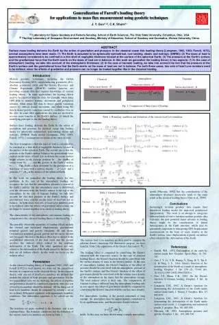
1. 2005 AGU fall meeting, 5-9 December 2005, San Francisco, USA Generalization of Farrell's loading theory for applications to mass flux measurement using geodetic techniques J. Y. Guo(1,2), C.K. Shum(1) (1)Laboratory for Space Geodesy and Remote Sensing, School of Earth Sciences, The Ohio State University, Columbus, Ohio, USA (2) The Key Laboratory of Geospace Environment and Geodesy, Ministry of Education, School of Geodesy and Geomatics, Wuhan University, China. ABSTRACT  Surface mass loading deforms the Earth by the action of gravitation and pressure. In the classical ocean tide loading theory [Longman, 1962, 1963; Farrell, 1972], several assumptions have been made: (1) The Earth is assumed to be spherically symmetrical, non-rotating, elastic and isotropic (SNREI); (2) The mass of load is approximately considered to be confined in a thin shell of negligible thickness located at the surface of the spherical Earth; (3) The pressure at the Earth’s surface and the gravitational force that the Earth exerts on the mass of load are in balance. In this work we generalize the loading theory in two aspects: (1) In the case of atmospheric loading, we take into account of the atmospheric thickness; (2) In the case of tsunami loading, we take into account the fact that the pressure at the Earth’s surface and the gravitational force that the Earth exerts on the mass of load are not in balance. For both these cases, two sets of load Love numbers need to be defined, since the effects of gravitation and pressure can no longer be treated together like in the classical loading. Introduction Modern geodetic techniques, including the Global Positioning System (GPS), superconducting gravimeter (SG), absolute gravimeter (AG) and the Gravity Recovery and Climate Experiment (GRACE) satellite mission, are providing accurate data that requires knowledge of various loading effects. In some applications, the loading effects need to be removed from the data, for example, when using GPS data to monitor tectonic movement and postglacial rebound, when using AG data to detect gravity variations caused by vertical crustal movement, and when using SG data to detect gravity variations caused by oscillatory flow in the core. In some other applications the data are inverted to recover mass transfer at the Earth’s surface, of which the underlying principle is also the loading theory. Surface mass loading deforms the Earth by the action of gravitation and pressure. In classical ocean tide loading theory for spherically symmetrical, non-rotating, elastic and isotropic (SNREI) Earth model [Longman, 1962, 1963; Farrell, 1972], 2 assumptions are made on the mass of load. The first assumption is that the mass of load is considered to be confined in a thin shell of negligible thickness located at the surface of the spherical Earth. The second one is that the pressure at the Earth’s surface balances the gravitational force exerted on the mass of load. Let us denote the ocean surface height relative to the average position by , the density of ocean water by , and the gravity at the Earth’s surface by . The Earth is then deformed by the gravitation of a thin layer of mass with a surface density , and a pressure at the surface of the spherical Earth. In this work we generalize the loading theory for two problems. In the case of the atmospheric loading, we recognize the fact that the atmospheric pressure is exerted at the Earth’s surface, but the atmospheric mass is distributed over the elevation from the Earth’s surface to the top of the atmosphere. In the case of tsunami loading, we take into account the fact that pressure at the Earth’s surface and gravitational force exerted on the mass of load are not in balance. In both cases, two sets of load Love numbers need to be defined, since the effects of gravitation and pressure can no longer be treated together as in classical loading theory. The characteristic of the atmospheric and tsunami loading in comparison to the classical loading theory is shown in Fig. 1. The possibly observable quantities of loading effects include the vertical and horizontal displacements, gravitational potential (geoid) and gravity variations, tilt and strain. Gravitational potential (geoid), gravity and tilt can be divided into two parts: the first is the direct effect that is related to the gravitational attraction of the load itself and the second involves the indirect effect related to the resulting deformation of the Earth. The other quantities are only related to the deformation of the Earth caused by the load and thus are all indirect effects. In this work we focus on the indirect effect. Formulation As the classical loading theory of Longman [1962, 1963] and Farrell [1972] is well known, we write out the generalized theories in comparison to the classical theory. In the classical theory, only one set of load Love numbers are defined that include the effects of both pressure and gravitation. For the two generalized cases we are studying, the effects of pressure and gravitation should be considered separately, thus two sets of load Love numbers should be defined. All the three sets of load Love numbers should be computed by solving a set of six ordinary differential equations with appropriate boundary conditions. The differential equations to be solved are the same: , The notations are quite standard in the literature, and is not explained here. The boundary conditions and the definition of the various load Love numbers are listed in Table 1. Atmospheric Tsunami Classical Volume mass density: Surface mass density: Surface mass density: Pressure: Pressure: Pressure: Fig. 1: Comparison of three types of loading Table 1: Boundary condition and definition of the various load Love numbers Boundary conditions Classical: Pressure: Gravitation: Load Love numbers Classical: Pressure: Gravitation: model [Merriam, 1992] that the consideration of the atmospheric thickness practically leads to the same result as the classical loading theory [Guo et al., 2004]. Conclusions Increasingly accurate geodetic data require finer theoretical loading model for improved geophysical interpretation.  This work is an attempt to categorize different kinds of load to interpret modern geodetic data. Certainly, the next potential major advance in loading theory might be the consideration of lateral heterogeneity in the Earth structure, which may be particularly important to interpreting GPS displacement measurements in the form of mass transfer at the Earth's surface, since displacement is purely an indirect effect related to the deformation of the Earth. Table 2: Green’s Function Classical: Pressure: Gravitation: Only is given for illustrative purpose. The various load Love numbers are then used to compute the relevant Green’s functions. For illustrative purpose, we have listed in Table 2 the expression of the Green’s function of . The loading effect is computed by convolving the Green’s function with the respective source. In the case of classical loading theory, the Green’s function should be convolved with the surface density of mass at the Earth’s surface. In the case of atmospheric loading, the Green’s function of the effect of pressure should be convolved with the atmospheric pressure at the Earth’s surface, and the Green’s function of the effect of gravitation should be convolved with the volume mass density of the atmosphere in the space that the atmosphere occupy. The total indirect effect is their sum. The computation of tsunami loading is different from the atmospheric loading only in one aspect: the effect of gravitation should be computed by convolving the Green’s function with the surface mass density. For atmospheric loading, if the period concerned is long enough, the atmosphere may be approximately considered to be at equilibrium state, and the pressure-density relation holds. In this case, we have shown using a simple atmospheric • References • Farrell, W.E., 1972. Deformation of the earth by surface loads, Rev. Geophys. Space Phys., 10, 761-797. • Guo, J. Y., Li, Y. B., Huang, Y., Deng, H. T., Xu, S. Q. & Ning, J. S., 2004. Green's function of the deformation of the Earth as a result of atmospheric loading. Geophys. J. Int. 159 (1), 53-68. doi: 10.1111/ j.1365-246X.2004.02410.x. • Guo, J.Y., Shum, C.K., 2005. On the Green's function of tsunami loading, Geophys. J. Int., In review. • Longman, I.M., 1962. A Green’s function for determining the deformation of the Earth under surface mass loads, 1. Theory, J. Geophys. Res., 67, 845-850. • Longman, I.M., 1963. A Green’s function for determining the deformation of the Earth under surface mass loads, 2. Computation and numerical results, J. geophys. Res., 68, 485-496. • Merriam, J.B., 1992. Atmospheric pressure and gravity, Geophys. J. Int., 109, 488-500.