Download
1 / 25
250 likes | 320 Views
Dive deep into the world of neural networks, exploring topics such as Perceptrons, Gradient Descent, Backpropagation, and Multi-layer Networks. Discover the inner workings of artificial and biological neural systems, learning through tuning connection weights. Suitable for those interested in machine learning, with a focus on problem domains, learning rules, and practical applications.

E N D
Machine Learning 2D5362 Artificial Neural Networks
Outline • Perceptrons • Gradient descent • Multi-layer networks • Backpropagation
Biological Neural Systems • Neuron switching time : > 10-3 secs • Number of neurons in the human brain: ~1010 • Connections (synapses) per neuron : ~104–105 • Face recognition : 0.1 secs • High degree of parallel computation • Distributed representations
Properties of Artificial Neural Nets (ANNs) • Many simple neuron-like threshold switching units • Many weighted interconnections among units • Highly parallel, distributed processing • Learning by tuning the connection weights
Appropriate Problem Domains for Neural Network Learning • Input is high-dimensional discrete or real-valued (e.g. raw sensor input) • Output is discrete or real valued • Output is a vector of values • Form of target function is unknown • Humans do not need to interpret the results (black box model)
ALVINN Drives 70 mph on a public highway Camera image 30 outputs for steering 30x32 weights into one out of four hidden unit 4 hidden units 30x32 pixels as inputs
x1 x2 xn Perceptron • Linear treshold unit (LTU) x0=1 w1 w0 w2 o . . . i=0n wi xi wn 1 if i=0nwi xi >0 o(xi)= -1 otherwise {
x2 + + + - - x1 + - - Decision Surface of a Perceptron x2 + - x1 + - • Perceptron is able to represent some useful functions • And(x1,x2) choose weights w0=-1.5, w1=1, w2=1 • But functions that are not linearly separable (e.g. Xor) • are not representable
Perceptron Learning Rule wi = wi + wi wi = (t - o) xi t=c(x) is the target value o is the perceptron output Is a small constant (e.g. 0.1) called learning rate • If the output is correct (t=o) the weights wi are not changed • If the output is incorrect (to) the weights wi are changed • such that the output of the perceptron for the new weights • is closer to t. • The algorithm converges to the correct classification • if the training data is linearly separable • and is sufficiently small
t=-1 t=1 o=1 w=[0.25 –0.1 0.5] x2 = 0.2 x1 – 0.5 o=-1 (x,t)=([2,1],-1) o=sgn(0.45-0.6+0.3) =1 (x,t)=([-1,-1],1) o=sgn(0.25+0.1-0.5) =-1 w=[0.2 –0.2 –0.2] w=[-0.2 –0.4 –0.2] (x,t)=([1,1],1) o=sgn(0.25-0.7+0.1) =-1 w=[0.2 0.2 0.2] Perceptron Learning Rule
Gradient Descent Learning Rule • Consider linear unit without threshold and continuous output o (not just –1,1) • o=w0 + w1 x1 + … + wn xn • Train the wi’s such that they minimize the squared error • E[w1,…,wn] = ½ dD (td-od)2 where D is the set of training examples
(w1,w2) Gradient: E[w]=[E/w0,… E/wn] (w1+w1,w2 +w2) Gradient Descent D={<(1,1),1>,<(-1,-1),1>, <(1,-1),-1>,<(-1,1),-1>} w=- E[w] wi=- E/wi =/wi 1/2d(td-od)2 = /wi 1/2d(td-i wi xi)2 = d(td- od)(-xi)
Gradient Descent Gradient-Descent(training_examples, ) Each training example is a pair of the form <(x1,…xn),t> where (x1,…,xn) is the vector of input values, and t is the target output value, is the learning rate (e.g. 0.1) • Initialize each wi to some small random value • Until the termination condition is met, Do • Initialize each wi to zero • For each <(x1,…xn),t> in training_examples Do • Input the instance (x1,…,xn) to the linear unit and compute the output o • For each linear unit weight wi Do • wi= wi + (t-o) xi • For each linear unit weight wi Do • wi=wi+wi
Incremental Stochastic Gradient Descent • Batch mode : gradient descent w=w - ED[w] over the entire data D ED[w]=1/2d(td-od)2 • Incremental mode: gradient descent w=w - Ed[w] over individual training examples d Ed[w]=1/2 (td-od)2 Incremental Gradient Descent can approximate Batch Gradient Descent arbitrarily closely if is small enough
Comparison Perceptron and Gradient Descent Rule Perceptron learning rule guaranteed to succeed if • Training examples are linearly separable • Sufficiently small learning rate Linear unit training rules uses gradient descent • Guaranteed to converge to hypothesis with minimum squared error • Given sufficiently small learning rate • Even when training data contains noise • Even when training data not separable by H
Multi-Layer Networks output layer hidden layer input layer
x1 x2 xn Sigmoid Unit x0=1 w1 w0 net=i=0n wi xi o=(net)=1/(1+e-net) w2 o . . . (x) is the sigmoid function: 1/(1+e-x) wn d(x)/dx= (x) (1- (x)) • Derive gradient decent rules to train: • one sigmoid function • E/wi = -d(td-od) od (1-od) xi • Multilayer networks of sigmoid units • backpropagation:
Backpropagation Algorithm • Initialize each wi to some small random value • Until the termination condition is met, Do • For each training example <(x1,…xn),t> Do • Input the instance (x1,…,xn) to the network and compute the network outputs ok • For each output unit k • k=ok(1-ok)(tk-ok) • For each hidden unit h • h=oh(1-oh) k wh,k k • For each network weight w,j Do • wi,j=wi,j+wi,j where wi,j= j xi,j
Backpropagation • Gradient descent over entire network weight vector • Easily generalized to arbitrary directed graphs • Will find a local, not necessarily global error minimum -in practice often works well (can be invoked multiple times with different initial weights) • Often include weight momentum term wi,j(n)= j xi,j + wi,j (n-1) • Minimizes error training examples • Will it generalize well to unseen instances (over-fitting)? • Training can be slow typical 1000-10000 iterations (use Levenberg-Marquardt instead of gradient descent) • Using network after training is fast
8-3-8 Binary Encoder -Decoder 8 inputs 3 hidden 8 outputs Hidden values .89 .04 .08 .01 .11 .88 .01 .97 .27 .99 .97 .71 .03 .05 .02 .22 .99 .99 .80 .01 .98 .60 .94 .01
Convergence of Backprop Gradient descent to some local minimum • Perhaps not global minimum • Add momentum • Stochastic gradient descent • Train multiple nets with different initial weights Nature of convergence • Initialize weights near zero • Therefore, initial networks near-linear • Increasingly non-linear functions possible as training progresses
Expressive Capabilities of ANN Boolean functions • Every boolean function can be represented by network with single hidden layer • But might require exponential (in number of inputs) hidden units Continuous functions • Every bounded continuous function can be approximated with arbitrarily small error, by network with one hidden layer [Cybenko 1989, Hornik 1989] • Any function can be approximated to arbitrary accuracy by a network with two hidden layers [Cybenko 1988]
Literature & Resources • Textbook: • ”Neural Networks for Pattern Recognition”, Bishop, C.M., 1996 • Software: • Neural Networks for Face Recognition http://www.cs.cmu.edu/afs/cs.cmu.edu/user/mitchell/ftp/faces.html • SNNS Stuttgart Neural Networks Simulator http://www-ra.informatik.uni-tuebingen.de/SNNS • Neural Networks at your fingertips http://www.geocities.com/CapeCanaveral/1624/ http://www.stats.gla.ac.uk/~ernest/files/NeuralAppl.html