Download
1 / 24
240 likes | 356 Views
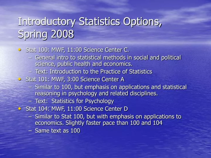
Introductory Statistics Options, Spring 2008. Stat 100: MWF, 11:00 Science Center C. General intro to statistical methods in social and political science, public health and economics. Text: Introduction to the Practice of Statistics Stat 101: MWF, 3:00 Science Center A

E N D
Introductory Statistics Options, Spring 2008 • Stat 100: MWF, 11:00 Science Center C. • General intro to statistical methods in social and political science, public health and economics. • Text: Introduction to the Practice of Statistics • Stat 101: MWF, 3:00 Science Center A • Similar to 100, but emphasis on applications and statistical reasoning in psychology and related disciplines. • Text: Statistics for Psychology • Stat 104: MWF, 11:00 Science Center D • Similar to Stat 100, but with emphasis on applications to economics. Slightly faster pace than 100 and 104 • Same text as 100
Overview • What can statistics be used for? • Our first quantitative example • Frequency tables • Graphical presentation of data: polygons, histograms, pie charts, bar charts • Types of Distributions • Summarizing Data – Central Tendency • Mean, Median, Mode • Summary
Chapter 1 • Statistics can be used to accomplish many different things – such as: • Quantification & measurement • Organizing and describing information • Systematic comparisons • Theoretical modeling • Weighing evidence and evaluating models
First Example How stressed have you been in the last 2 ½ weeks? Scale: 0 (not at all) to 10 (as stressed as possible) 4 7 7 7 8 8 7 8 9 4 7 3 6 9 10 5 7 10 6 8 7 8 7 8 7 4 5 10 10 0 9 8 3 7 9 7 9 5 8 5 0 4 6 6 7 5 3 2 8 5 10 9 10 6 4 8 8 8 4 8 7 3 7 8 8 8 7 9 7 5 6 3 4 8 7 5 7 3 3 6 5 7 5 7 8 8 7 10 5 4 3 7 6 3 9 7 8 5 7 9 9 3 1 8 6 6 4 8 5 10 4 8 10 5 5 4 9 4 7 7 7 6 6 4 4 4 9 7 10 4 7 5 10 7 9 2 7 5 9 10 3 7 2 5 9 8 10 10 6 8 3 from Aron & Aron’s text, Statistics for Psychology
Frequency Tables • A frequency table shows how often each value of the variable occurs
Frequency Polygon • A visual representation of information contained in a frequency table • Align all possible values on the bottom of the graph (the x-axis) • On the vertical line (the y-axis), place a point denoting the frequency of scores for each value • Connect the lines • (Typically add an extra value above and below the actual range of values)
Histograms • Another way of visually representing information contained in a frequency table • Histograms are kind of like bar charts; bars are used instead of connected points • The bars typically cover “intervals” of values. The first bar here covers scores > 0 and < 1.
Pie Charts and Nominal Data • Pie charts are commonly used to represent the frequency of scores for nominal data • Here, frequency of referents in a letter written by a subject in a psychological study. • 70% of the pronouns are in reference to the writer; 10% are in reference to the person being written to.
Barcharts and Nominal Data • Barcharts are sometimes used to represent the frequency of scores for nominal data • Here, frequency is expressed as a percentage of the total number of males and females • (78% and 68%)
Shapes of Distributions • These representational aides all describe frequency distributions: the way score frequencies are distributed with respect to the values of the variable • Distributions can take on a number of shapes or forms
Unimodal Distributions • The mode of a distribution refers to the most frequently occurring score • In a unimodal distribution, one score occurs much more frequently than others
Multimodal Distributions • In multimodal distributions, more than one mode exists (or approximately so) • In a bimodal distribution, two modes exist
Rectangular or Uniform Distributions • In a uniform distribution, all values are observed equally often
Symmetrical and Skewed Distributions • A symmetrical distribution is balanced: if we cut it in half, the two sides would be mirror images of one another • normal distribution: a particular kind of distribution that resembles a bell (bell-shaped distribution)
Skewed Distributions • A skewed distribution is unbalanced; there may be a cluster of scores piling on one end of the scale
Skew negative skew positive skew reasons for skew?
Question How can we summarize a distribution of scores efficiently using quantitative (as opposed to graphical) methods?
Measures of Central Tendency • Central tendency: most “typical” or common score (a) Mode (b) Median (c) Mean
Measures of Central Tendency 1. Mode: most frequently occurring score 10, 20, 30, 40, 40, 50, 60 Mode = 40
Measures of Central Tendency 2. Median: the value at which 1/2 of the ordered scores fall above and 1/2 of the scores fall below 1 2 3 4 5 1 2 3 4 Median = 3 Median = 2.5
Measures of Central Tendency x = an individual score N = the number of scores Sigma or = take the sum • Note: Equivalent to saying “sum all the scores and divide that sum by the total number of scores” 3. Mean: The “balancing point” of a set of scores; the average
(-2) (+4) (-2) (– 1) + (– 2) + (– 2) + 1 + 4 = 0 B A C D E 3 4 5 6 7 8 9 (+1) (-1)
(– 1) + (– 3) + (– 4) + (– 4) + 2 = –10 B A C D E 3 4 5 6 7 8 9 (-1) (-3) (+2) (- 4) (- 4)
Summary • What can statistics be used for? • Our first quantitative example • Frequency tables • Graphical presentation of data: polygons, histograms, pie charts, bar charts • Types of Distributions • Summarizing Data – Central Tendency • Mean, Median, Mode