Gene Finding Approaches
Gene Finding Approaches. L529 Presentation (Nov 17, 2003) Xin Hong , Yi Zou and Xiang Zhou. Outline. Part I Overview of gene finding approaches Part II GENSCAN Part III TWINSCAN and GLASS-ROSETTA Part IV Evolutionary Hidden Markov Model. Introduction.

Gene Finding Approaches
E N D
Presentation Transcript
Gene Finding Approaches L529 Presentation (Nov 17, 2003) Xin Hong, Yi Zou and Xiang Zhou
Outline • Part I Overview of gene finding approaches • Part II GENSCAN • Part III TWINSCAN and GLASS-ROSETTA • Part IV Evolutionary Hidden Markov Model
Introduction Genome Project Gene Prediction Proteomics
Difference between Prokaryotic and Eukaryotic Genomes (adopted from Sanja Rogic’s Jan 23 2003 talk. CS Department UBC)
Difference between Prokaryotic and Eukaryotic Genomes Prokaryotes: • small genomes 0.5 – 10·106 bp • High coding sequence density (i.e. in yeast genome, 75% is coding sequences) • Introns are either non-existent or short. Eukaryotes: • large genomes 107 – 1010 bp • Very low coding sequence density. Exons are scattered in a vast sea of non-genic ‘noise’. (i.e. in human genome, only ~ 3% are coding seqs) • Alternative splicing sites
Eukaryotic Gene Structure 5’ - Promoter Exon1 Intron1 Exon2 Terminator – 3’ UTR splice splice UTR (adopted from Amir Mitchell’s talk) transcription Poly A translation protein
Prokaryotic Gene Structure (adopted from Amir Mitchell’s talk) Promoter CDS Terminator UTR UTR Genomic DNA transcription mRNA translation protein
Gene Finding Given a genomic sequence or a set of genomic sequences, find out: • Exons (coding exons) • Introns • Splicing sites • Regulatory sequences (5’-UTR, 3’-UTR, promoter, polyA tails)
Gene Finding Approaches • Ab initio methods i.e. GENSCAN (Burge C. 1997), GENIE (Reese M. et al. 2000) , TWINSCAN (Korf I. et al 2001) • Homology search methods i.e. PROCRUSTES (Gelfand S. et al. 1996), GENEWISE (Birney E) • Comparative search methods i.e. GLASS-ROSETTA (Batzoglou S. et al. 2000), EHMM (Pederson JS and Hein J, 2003)
Ab initio methods • Use the DNA sequence • Use a gene structure model which includes information of: - splice donor & acceptor sites, - start and stop codons, - promoter features such as TATA boxes, TF binding sites, CpG islands
Homology search methods • First used by Staden and McLachlan in 1982 • Use local alignment tools (Smith-Waterman algorithm, BLAST, FASTA) to search databases for homologs • Accuracy of prediction depends on the presence of homologs in the databases
Comparative search methods • Align genomic sequences from related species • Involve evolutionary information • Two comparative methods - Simultaneous alignment and gene structure prediction (i.e. GLASS-ROSETTA) - Gene structure prediction based on given alignment (i.e. Evolutionary Hidden Markov Model)
GenScan • GENSCAN is a computer program for gene identification • Developed by Chris Burge (Burge 1997), Stanford University. • J.Mol. Biol.(1997) 268: 78-94 • One of the most accurate ab initio programs
Genscan Server http://genes.mit.edu/GENSCAN.html
GenScan Characteristics Designed to predict complete gene structures • Introns and exons, Promoter sites, Polyadenylation signals • Incorporates: • Descriptions of transcriptional, translational and splicing signal • Length distributions (Explicit State Duration HMMs) • Compositional features of exons, introns, intergenic, C+G regions • Larger predictive scope • Deal with partial and complete genes • Ability to predict multiple genes in a sequence • Ability to predict consistent sets of genes occurring on either or both strands of the DNA.
Genscan Model • It is based on Generalized HMM (GHMM) • Model both strands at once
N - intergenic region P - promoter F - 5’ untranslated region Esngl – single exon (intronless) (translation start -> stop codon) Einit – initial exon (translation start -> donor splice site) Ik – phase k intron: 0 – between codons; 1 – after the first base of a codon; 2 – after the second base of a codon Ek – phase k internal exon (acceptor splice site->donor splice site) Eterm – terminal exon (acceptor splice site -> stop codon) T - 3’ untranslated region A – poly-A GenScan States
Four main components of model: • A vector of initial state probability distribution, • A matrix of state transition probabilities T • A set of length distributions ƒ for different states • A set of sequence generating models P for each of the states
GenScan model parameters • Uses as a training set 238 multi-exon genes and 142 single-exon genes from GenBank to compute parameters • Initial state probabilities • Transition probabilities • State length distributions • Probabilistic models for the states • The states correspond to different functional units on a gene e.g promoter regions, exon • Transitions ensure that the order that the model marches through the states is biologically consistent • Length distributions take into account that different functional units have different lengths.
Initial and transition probability Based on CG content, initial and transition probability distribution are estimated in each of four categories: I (<43% C+G); II(43-51);III(51-57); and IV (>57). To simplify the model, the initial probabilities of the exon, polyadenylation signal and promoter states are set to zero.
State length distribution • Intron and intergenic length are modeled as geometric distribution with parameter q estimated for each C+G group. • 5-UTR and 3-UTR with mean value of 769 and 457 bp by geometric distribution • Exon length L=3c+i(c is the number of complete codon,i is the phase of subsequent intron: 0,1 or 2)
State Models • Coding regions: inhomogeneous 3-periodic fifth-order Markov model (Borodovsky & Mcininch, 1993,Comp.Chem. 17,123-133) • Non-coding states (introns, 5’UTR, 3’UTR, intergenic regions): homogeneous fifth-order Markov model
Signal models used by GenScan • WMM= weight matrix model (Staden, 1984, Nucl. Acids Res, 12, 505-519) • For transcriptional and translational signals (translation initiation, polyA signals, TATA box etc.) • polyA signal is modeled as a 6 bp WMM with AATAAA as the consensus sequence (uses annotated data from GenBank) • WAM= weight array model (Zhang & Marr, 1993, Comp. Appl.Biol.Sci.9(5): 499-509) • Assumes some Dependencies between adjacent positions in the sequence • used for the pyrimidine-rich region and the splice acceptor site • MDD=Maximal dependency decomposition model (Burge, 1997, J.Mol. Biol. 268: 78-94) • used for donor splice sites
Transcription and translation signal • Translation initiation signal: 12bp WMM model with 6bp as start codon. • Translation termination signal: one of the three stop codons is generated and the next three nucleotides are generated according to a WMM. • Promotor model: TATA-containing promotor with probability 0.7 and TATA-less promotor with probability 0.3 because 30% eukaryotic organisms don’t have TATA signal. • TATA-containing promoter is modeled using a 15 bp TATA-box WMM and an 8 bp cap site WMM. • TATA-less promoters are modeled simply as intergenic-null regions of 40 bp in length.
Application of model • A precise probabilistic model of what a gene/genomic sequence looks like is specified in advance. • Then, determine which of the vast number of possible gene structure has highest likelihood given a sequence
Predicting the Gene Structure Genscan model, essentially semi-Markov type, can be formulated as an explicit state duration HMM, The model generate “parse” Ф: • An ordered set of states q = {q1,q2,…,qn} • An Associated set of length (duration) d={d1,d2,…,dn} • Using probabilistic models of each of the state types, generate a DNA sequences S of length L=∑di (I=1...n)
Generating a parse corresponding to a sequence length L: • Choose initial q1 according to an initial distribution on the states π. • A length (state duration), d1, corresponding to the state q1 is generated conditional on the value from the length distribution fQ. • According to an appropriate sequence generating model for state type q1,generate a sequence segment s1 of length d1 based on d1 and q1. • The subsequent state q2 is generated, based on the value of q1, from the state (first-order Markov) transition matrix T. This process is repeated until the sum of the state duration first equals or exceeds the length L. The sequence generated is the concatenation of the sequence segments, S=s1,s2…Sn.
Prediction • Given a sequence, find the most probable gene structure compatible with the sequence • For a particular sequence S, the conditional probability of a particular parse Φ using Bayes’ Rule is:
Algorithm • Find the most probable parse, opt, using a Viterbi-like algorithm • Find P(S) using a “forward” algorithm • Run time: at worst, quadratic in the number of possible state transitions • In practice grows approximately linearly with sequence length for sequences of several kb or more
TWINSCAN • TWINSCAN is developed by Brent’s group in Washington University, 2001. - TWINSCAN Website http://genes.cs.wustl.edu/ - Original paper Korf, I., P. Flicek, D. Duan, and M.R. Brent. 2001. Integrating genomic homology into gene structure prediction. Bioinformatics 17: S140-148.
TWINSCAN • Reason for developing TWINSCAN - GENSCAN performed poorly on the HTG sequences. • What is HTG sequences? - high-throughput genomic sequences - usually 100-200kb in length, - contain an unknown number of genes • TWINSCAN is designed specifically for HTG sequences
TWINSCAN • Based on GENSCAN • Different from GENSCAN - GENSCAN model does not account for evolutionary conservation. - TWINSCAN extends the probability model of GENSCAN and utilize the pattern of evolutionary conservation.
TWINSCAN • Use the GENSCAN model topology for parsing. c-state d-state E0 E1 E2 I0 I1 I2 Einit Eterm 3’ UTR 5’ UTR Esngl polyA P N
Component models of c-states - Fifth Order Markov Chain - Weight Matrix Model (WMM) - Weight Array Model (WAM) - Maximal Dependence Decomposition (MDD) - Conservation Models
Conservation Sequence • Conservation symbolic representation . unaligned, | matched, : mismatched i.e. 1 2 3 45 67 8 9 position GAATTCCGT target sequence alignment 3 45 67 8 9 target position ATT- CCGT target alignment | | | | | alignment match symbols ATCACC- T informant alignment the resulting conservation sequence is 1 2 3 45 67 8 9 position GAATTCCGT target sequence . . | | : | | : | conservation sequence
TWINSCAN • State-specific sequence model combines - the probability model of generating a specific DNA sequences from any given state. - the probability model of generating a conservation sequence from any given state. • Possible states - Coding state, UTR state, intron/intergenic state - translation initial and termination sites - splicing donor and acceptor sites • For instance, given from i to j is an exon Pr( Ti, j, Ci,j| Ei, j ) = Pr(Ti, j| Ei, j ) Pr(Ci, j| Ei, j )
TWINSCAN vs GENSCAN Compare to GENSCAN, TWINSCAN shows notable improvement in exon sensitivity and specificity and dramatic exact gene sensitivity and specificity.
GLASS-ROSETTA • GLASS-ROSETTA is developed by Berger’s group in MIT, 2000 • Original paper is "Human and mouse Gene Structure: Comparative Analysis and Application to Exon Prediction."Genome Research, July 1, 2000. • Web Interface http://crossspecies.lcs.mit.edu/ • ROSETTA is the first program for gene prediction based on cross-species comparison of genomic DNA from two organisms.
GLASS-ROSETTA How to identify exons directly from cross-species comparison of genomic DNA?
GLASS-ROSETTA • Analyze the genomic structure of the training data set which contains 117 orthologous gene pairs from human and mouse • Get conservation information - splice sites - exon number: 95% identical - exon length: 73% identical - coding frame - sequence similarity: 85% identical • Develop the algorithms for GLASS and ROSETTA
GLASS-ROSETTA • GLASS (GLobal Alignment SyStem) - is a tool for aligning pairs of homologous sequences. It is designed for aligning long, divergent sequences, that contain blocks of moderate to strong homology, such as orthologous/paralogous pairs of genes. • ROSETTA - is a tool for predicting coding exons on a target human sequence (may also work for other mammalian sequences as targets), based on comparison with a homologous sequence from a different species (adopted from GLASS-ROSETTA WEBSITE)
GLASS-ROSETTA Align two genomic sequences using GLASS Process aligned sequences to mask repeats (using Repeat-Masker) and poorly aligned regions Annotate genes using ROSETTA
The goal of ROSETTA is to find the optimal parse • A “parse” of a genomic region is a sequence ([a1,b1, t1, s1, f1], [a2, b2, t2, s2, f2],. . . [an, bn, tn, sn, fn]) • ei = (ai , bi, ti, si, fi) denotes consecutive exons with - starting and stopping points (ai, bi) - type ti {ini-tial, internal, terminal} - designated strand si { +, -} - reading frame fi {0,1,2}. 5’ - Promoter Exon1 Exon2 Exon3 Terminator – 3’ UTR Intron1 Intron2 UTR
The goal of ROSETTA is to find the optimal parse n Score (parse) = ∑score [parse (i)] i=1 • The score for each coding exon consisted of several components - splice sites scores are calculated by using a hybrid method that combines the GENSCAN splice site detector and a directionality effect. - codon usage scores are calculated by summing the log odds ratio for each codon, based on published codon frequencies for the organism. - amino acid smilarity scores are calculated by comparing corresponding codons in the two exons and ususing the PAM20 matrix to score matches, mismatches and gaps. - exon length scores
ROSETTA • Performed extremely well at identifying internal coding exons. • Somewhat less accurate for initial and terminal coding exons. • Compare to GENSCAN: Similar at sensitivity (95% vs 98%). Bbetter specificity (97% vs 89%)