Download
1 / 17
170 likes | 364 Views
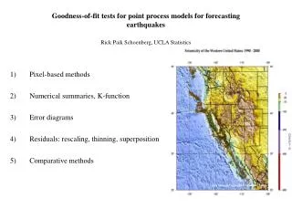
Goodness-of-fit tests for point process models for forecasting earthquakes Rick Paik Schoenberg, UCLA Statistics. 1) Pixel-based methods 2) Numerical summaries, K-function 3) Error diagrams 4) Residuals: rescaling, thinning, superposition 5) Comparative methods.

E N D
Goodness-of-fit tests for point process models for forecasting earthquakes Rick Paik Schoenberg, UCLA Statistics 1) Pixel-based methods 2) Numerical summaries, K-function 3) Error diagrams 4) Residuals: rescaling, thinning, superposition 5) Comparative methods
A few examples of some commonly-used conditional intensity models in seismology: • Stationary (homogeneous) Poisson process: (t,x) = . • Inhomogeneous Poisson process: (t, x) = f(t, x). (deterministic) • ETAS (Epidemic-Type Aftershock Sequence, Ogata 1988, 1998): • (t, x) = (x) + ∑ g(t - ti, ||x - xi||, mi), • ti < t • where g(t, x, m) = K exp{m} • (t+c)p (x2 + d)q
1. Pixel-based methods.Compare N(Ai) with ∫A(t, x) dt dx, on pixels Ai. (Baddeley, Turner, Møller, Hazelton, 2005)Problems:* If pixels are large, lose power.* If pixels are small, residuals are mostly ~ 0,1.* Smoothing reveals only gross features.
2. Numerical summaries.a) Likelihood statistics (LR, AIC, BIC). Log-likelihood = ∑ log(ti,xi) - ∫ (t,x) dt dx.b) Second-order statistics. * K-function, L-function (Ripley, 1977) * Weighted K-function (Baddeley, Møller and Waagepetersen 2002, Veen and Schoenberg 2005) * Other weighted 2nd-order statistics: R/S statistic, correlation integral, fractal dimension (Adelfio and Schoenberg, 2009)
Weighted K-function Usual K-function: K(h) ~ ∑∑i≠j I(|xi - xj| ≤ h), Weight each pair of points according to the estimated intensity at the points: Kw(h)^~ ∑∑i≠j wi wj I(|xi - xj| ≤ h), where wi = (ti , xi)-1. (asympt. normal, under certain regularity conditions.) Lw(h) = centered version = √[Kw(h)/π] - h, for R2
2. Numerical summaries.a) Likelihood statistics (LR, AIC, BIC). Log-likelihood = ∑ log(ti,xi) - ∫ (t,x) dt dx.b) Second-order statistics. * K-function, L-function (Ripley, 1977) * Weighted K-function (Baddeley, Møller and Waagepetersen 2002, Veen and Schoenberg 2005) * Other weighted 2nd-order statistics: R/S statistic, correlation integral, fractal dimension (Adelfio and Schoenberg, 2009) c) Other test statistics (mostly vs. stationary Poisson). TTT, Khamaladze (Andersen et al. 1993) Cramèr-von Mises, K-S test (Heinrich 1991) Higher moment and spectral tests (Davies 1977) Problems: -- Overly simplistic. -- Stationary Poisson not a good null hypothesis (Stark 1997)
3. Error DiagramsPlot (normalized) number of alarms vs. (normalized) number of false negatives (failures to predict). (Molchan 1990; Molchan 1997; Zaliapin & Molchan 2004; Kagan 2009).Similar to ROC curves (Swets 1973).Problems: -- Must focus near axes. [consider relative to given model (Kagan 2009)] -- Difficult to see where model fits poorly.
4. Residuals: rescaling, thinning, superposing Rescaling. (Meyer 1971;Berman 1984; Merzbach &Nualart 1986; Ogata 1988; Nair 1990; Schoenberg 1999; Vere-Jones and Schoenberg 2004): Suppose N is simple. Rescale one coordinate: move each point {ti, xi} to {ti , ∫oxi(ti,x) dx} [or to {∫oti(t,xi) dt), xi }]. Then the resulting process is stationary Poisson. Problems: * Irregular boundary, plotting. * Points in transformed space hard to interpret. * For highly clustered processes: boundary effects, loss of power.
Thinning. (Westcott 1976):Suppose N is simple, stationary, & ergodic.
Thinning: Suppose inf (ti ,xi) = b. Keep each point (ti ,xi) with probability b / (ti ,xi) . Can repeat many times --> many stationary Poisson processes (but not quite ind.!)
Superposition. (Palm 1943): Suppose N is simple & stationary. Then Mk --> stationary Poisson.
Superposition: Suppose sup (t, x) = c. Superpose N with a simulated Poisson process of rate c - (t, x) . As with thinning, can repeat many times to generate many (non-independent) stationary Poisson processes. Problems with thinning and superposition: Thinning: Low power. If b = inf (ti ,xi) is small, will end up with very few points. Superposition: Low power if c = sup (ti ,xi) is large: most of the residual points will be simulated.
5. Comparative methods. -- Can consider difference (for competing models)between residuals over each pixel. Problem: Hard to interpret. If difference = 3, is this because model A overestimated by 3? Or because model B underestimated by 3? Or because model A overestimated by 1 and model B underestimated by 2? Also, when aggregating over pixels, it is possible that a model will predict the correct number of earthquakes, but at the wrong locations and times. -- Better: consider difference between log-likelihoods, in each pixel. Problem: pixel choice is arbitrary, and unequal # of pts per pixel…..
Conclusions: * Point process model evaluation is still an unsolved problem. * Pixel-based methods have problems: non-normality, high variability, low power, arbitrariness in choice of pixel size. Comparing log-likelihoods within each pixel seems a bit more promising. * Numerical summary statistics and error diagrams provide very limited information. * Rescaling, thinning, and superposition also have problems: can have low power, especially when the intensity is volatile.