Game Theory and Business Strategy Part I

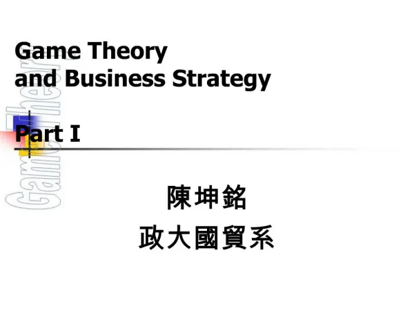
Game Theoryand Business Strategy Part I 陳坤銘政大國貿系

Game Theoryand Business Strategy Part I Lecture 5 Simultaneous-Move Games with Pure Strategies II: Continuous Strategies and III: Discussion and Evidence

Outline • Continuous pure strategies • Empirical evidence concerning Nash equilibrium • Critical discussion of the Nash equilibrium concept • Rationalizability

Continuous Pure Strategies • When players have a large range of actions available, game tables become virtually useless as a analytical tools. • The continuity of the sets of strategies allows us to show the best responses as curves in a graph, with each player’s strategy on one of the axes. • The Nash eq. occurs where the two curves meet.,

Restaurant Pricing Game Yvonne’s price Py Xavier’s best response Px=15+0.25Py Two restaurants: Yvonne (x) & Xavier (y) Qi=44-2Pi+Pi Ci=8 Bi=(Pi-8)*Qi 30 Joint best Yvonne’s best response Py=15+0.25Px 20 Nash equilibrium 10 Xavier’s price Px 10 20 30 Figure 5.1 Best-response curves and equilibrium in the restaurant pricing game

Pricing Game (con’t) • This pricing game is exactly like the prisoners’ dilemma game. They can raise their profits if they cooperatively agree to raise their prices. • Collusion need not always lead to higher prices. If two firms sell products that are complements to each other, then allowing them to cooperate would lead to lower prices and thus be beneficial to the consumers as well.

Party R’s ad, y ($millions) 1 Party L’s best response X= y^(1/2)-y Nash equilibrium Party R’s best response y= x^(1/2)-x 0.25 Party L’s ad, x ($millions) 0 0.25 1 Campaign Advertising Game Two parties: R and L Advertising expenditures of R and L: y and x Vote shares of R and L: y/(x+y) and x/(x+y) Payoffs of R and L: y/(x+y) –y and x/(x+y)-x Figure 5.2 Best responses and Nash equilibrium in the campaign advertising game

Campaign Advertising Game(con’t) • As in the pricing game, we have a prisoners’ dilemma in campaign advertising game. If both parties cut back on their ads in equal proportions, their vote shares would be entirely unaffected, but both would save on their expenditures and so both would have a larger payoff. • Like a producer’s cartel for complements, a politicians’ cartel to advertise less would probably benefit voters and society.

Evidence from Laboratory and Classroom Experiments • Choosing among multiple equilibria • Players generally fail to coordinate unless they have some common cultural background (and this fact is common knowledge among them) that is needed for locating focal points.

Evidence from Laboratory and Classroom Experiments • Revelation of innate altruism or public-spiritedness in experiments • People seem to “err” on the side of niceness or fairness. The reason might be that the players’ payoffs are different from those assumed by the experimenter.

Real-World Evidence • Explanatory power • There are numerous successful examples of using game-theoretical reasoning to explain phenomena that are observed in reality. • Examples including international relations, firm behavior, auctions, voting, and bargaining.

Real-World Evidence • Statistical testing • Game-theoretical models fit the data to many major industries reasonably well. • In politics, game-theoretical models have been used successfully in explaining the voting behavior of U.S. legislators.

Real-World Evidence • A real-world example of learning • Throughout 20th century the best batting averages recorded in a baseball season have been declining, along with overall decrease in variation. • Gould argues that through a succession of adjustments of strategies to counter one another, the system settled down into its Nash equilibrium.

Implications of Empirical Evidence • On the whole, one should have considerable confidence in using the Nash equilibrium concept when the game in question is played frequently by players from a reasonably stable population and under relatively unchanging rules and conditions.

Implications of Empirical Evidence • When the game is new or is played just once and the players are inexperienced, one should use the equilibrium concept more cautiously and should not surprised if the outcome is not consistent with that the theory predicts.

A game with a questionable Nash equilibrium • Unique Nash equilibrium (C1, R1) • However, playing C3 has a lot of appeal, because it guarantees you the same payoff as you would get in the Nash eq. Figure 5.3 A game with a questionable Nash equilibrium

A game with a questionable Nash equilibrium (Con’t) • But, note that if you really believe that the other player would play C, then you should play B to get the payoff 3. And if you think the other person would think thus and so would play B, then your best response to B is A. And if you think the other would figure this out too, you should be playing your best response to A, namely A. Back to the Nash equilibrium. Figure 5.3 A game with a questionable Nash equilibrium

Disastrous Nash Equilibrium • Unique Nash equilibrium:: (Down, Left) • If A has any doubts about either B’s payoffs or B’s rationality, the it is a lot safer for A to play Up than to play her Nash equilibrium strategy of Down. A thinks there is a probability p that B plays Right. 1-p p Figure 5.4 Disastrous Nash equilibrium

Disastrous Nash Equilibrium (Con’t) • However, if there is any doubts about B’s payoffs, then the fact should be made an integral part of the analysis. It is better for A to choose UP if 9(1-p)+8p > 10(1-p)-1000p or p > 1/1009 Figure 5.4 Disastrous Nash equilibrium

Multiplicity of Nash Equilibria • Many games have multiple Nash equilibria. • Nash equilibra may fail to pin down outcomes of games sufficiently precisely to give unique predictions. • Nash equilibrium concept is not enough by itself and must be supplemented by some other consideration that selects the one equilibrium with better claims to be the outcome than the rest.

Justifying choices by chains of beliefs and responses • A strategy that is strictly dominated is never a best response. However, a strategy might never be a best response even though it is not strictly dominated. • The strategy that remains after the iterative deletion of strategies that are never a best response is known as a rationalizable strategy.

Justifying choices by chains of beliefs and responses • Unique Nash eq.: (R2, C2) • In the matrix of Figure 5.5, we can justify any pair of strategies. Thus, rationality alone does not justify Nash eq. Figure 5.5 Justifying choices by chains of beliefs and responses

Justifying choices by chains of beliefs and responses (con’t) • For instance, we can justify Row’s choice of R1, since R1 is Row’s best choice if she believes Column is choosing C3. • The reason that she believes that Column is choosing C3 is that she believes that Column believes that Row is playing R3. • Row justifies this belief by thinking that Column believes that Row believes that Column is playing C1, believing that Row is playing R1, believing in turn… Figure 5.5 Justifying choices by chains of beliefs and responses

Applying the concept of Rationalizability (con’t) Never a best response • Note that C4 is never a best response, but it is not dominated by other strategies. • Since R4 is Row’s best response only against C4, Column should never believes that Row will play R4. Never a best response Figure 5.6 Rationalizable Strategies

Applying the concept of Rationalizability (con’t) • Even if a game does not have a Nash eq., it may have rationalizable outcomes. • Rationalizability provides a possible way of solving games that do not have a Nash equilibrium. • More importantly, the concept tells us how far we can narrow down the possibilities in a game on the basis of rationality. Figure 5.6 Rationalizable Strategies

y 30 BR1: x=15-y/2 12 N=(12,6) 7.5 BR2: y=12-x/2 4.5 x 0 9 15 13.75 24 Nash equilibrium through Rationalizability The Nash equ. is the only outcome that survives the iterated elimination of strategies that are never best responses. Two boat owners: U and V The strategies of U and V: x and y Fishing costs of U and V: 30 and 36 The price P will be P=60-(x+y) Profit of U and V: U = [(60-x-y)-30]x V = [(60-x-y)-36]y Figure 5.7 Nash equilibrium through rationalizability

Nash equilibrium through Rationalizability(con’t) • The whole range of the second owner’s best responses is between 0 and 12. Similarly, the second owner cannot rationally think that the first owner will produce anything less than 0 or greater 15. • Now take this to the second round. When the first owner has restricted the second owner’s choices of Y to {0,12}, her own choices of X are changed to {0,9} accordingly. Similarly, the second owner’s choices of Y are changed to {0, 4.5}. Figure 5.6 Rationalizable Strategies

Nash equilibrium through Rationalizability(con’t) • The third round of thinking narrows the ranges further. This succession of rounds can be carried as far as you like. • It is evident that the successive narrowing of the two ranges is converging on the Nash equilibrium. Figure 5.6 Rationalizable Strategies

Game Theory and Business Strategy Part I