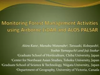
Monitoring Forest Management Activities using Airborne LiDAR and ALOS PALSAR

1. Monitoring Forest Management Activities using Airborne LiDAR and ALOS PALSAR Akira Kato1, Manabu Watanabe2, Tatsuaki, Kobayashi1, Yoshio Yamaguchi3,and Joji Iisaka4 1Graduate School of Horticulture, Chiba University, Japan 2Center for Northeast Asian Studies, Tohoku University, Japan 3Graduate School of Science & Technology, Niigata University,, Japan 4Department of Geography, University of Victoria, Canada

2. ALOS PALSAR ⇔Airborne LiDAR • ALOS PALSAR - L-band radar →　polarization (indirect measurement) - Multi-temporal data - Lowcost - Globalacquisition - 15m～ resolution→　plot level estimation • Airborne LiDAR - Near-infrared red laser →　direct measurement - (Multi-) temporal data - Highcost - Local acquisition - 10cm ～　resolution→ single tree level estimation

3. Problem ⇒ study frame ALOS PALSAR ⇔ limited field samples • Bottom-up approach State Level: Biomass change is monitored using PALSAR as same quality as global scale. District Level: Biomass change is monitored using Airborne LiDAR Stand Level: Biomass change is monitored using Airborne or terrestorialLiDAR

4. Forest Biomass ⇔ Volume Scattering • Past studies 1. Saturation level of forest biomass using L-band 100 ton/ha in homogeneous pine forest (Imhoffet al., 1995) ⇒　Approx. 5meters spacing of 20 m height trees. 40 ton/ha in broadleaf evergreen forest (Lucas et al., 2006) 2. HV polarization is higher correlation with forest biomass (Lucas et al., 2006) ALOS PALSAR is a good sensor to detect the forest management activities, but correlation between backscattering coefficient and the change is still unknown.

5. Volume Scattering ⇔stand condition • Stand condition is defined by - stem density - tree height - tree forms (the shape of tree crown) - tree age ⇒ airborne LiDARis used to bridge between field measurement and backscattering coefficient of ALOS PALSAR as the ground truth.

6. Study frame ⇒forest management activities • ２０１０Summer ALOS PALSAR data after thinning The second airborne LiDARacquisiton • ２００９ Summer ALOS PALSAR data before thinning The first airborne LiDARacquisiton Wider scale biomass change Ground Truth Continuous samples modeling Discrete samples field work - measure trees. • ２００９& ２０１０Ｗｉｎｔｅｒ We thinned trees.

7. Terrestrial LiDAR (after thinning)

8. Study Area • Sanmu City, Chiba Prefecture, JAPAN → Commercial timber production area • Research area is around 9 km2 • - Dominant species is Japanese cedar • (Cryptomeria japonica) • Homogeneous stands • - 30 plots (20m x 20m) were set

9. Data – Airborne LiDAR HH HV Before thinning After thinning

10. Data – ALOS PALSAR L-band FBD (Fine beam Double Polarization) Resolution: 20m • ALOS satellite endedat May 2011. • - 20 m resolution L-band SAR. • - 46 days observation cycle. • ALOS 2 will be launched at 2013. • 1～3 m resolution L-band SAR. • 16 days observation cycle. Before thinning After thinning Backscattering coefficient - σ0(dB, amplitude value) HH HV

11. Preprocessing – ALOS PALSAR １．Geometric and terrain correction ⇒MapReady (Alaska Satellite Facility, ver 2.3, 2010). 2. layover / shadow regions for the terrain correction 　　⇒5m resolution DEM provided by Geospatial Information Authority of Japan 3. Speckle filtering ⇒Averaging the values of multi-temporal data. The data before thinning (before August 2010) and after thinning (after August 2010) are averaged separately. 4. Pixel alignment ⇒Manual geo-referencing was applied to match the images with less than half pixel of error (10m) among the multi-temporal data

12. Preprocessing – Airborne LiDAR Digital Terrain Model Digital Canopy Model ⇒Tree Top location Digital Surface Model

13. Preprocessing DSM (50cm) DTM (50cm) Thinned area ⇒ white 2010 DCM (50cm)

14. Methodology – Identify Tree Tops • Stem height and location have been identified by (Bloomenthal et al., 1997) Second order Taylor’s approximation

15. Tree top location and height Before Thinning (Aug 2009) After Thinning (July 2010) m

16. Methodology • Biomass estimation Biomass = (stem volume = f (tree height, dbh)) × (density factor) ×(expansion factor of branch) ×(expansion factor of stem) Stem volume = α(stem density) +β(tree height) + C

17. Results and Discussion Airborne LiDAR Stem density Tree height Stem density correction: y = 2.5034x - 12.41 where x: the number of stems derived from airborne lidar y: the corrected number of stems

18. Results and Discussion V = 20.94 log(N) + 82.94 log(H) - 113.10 m m

19. Stem Volume Change (m3) HH HV High: 137.03 Low: -116.04 m

20. Results and Discussion • HV/HH is shifted in 9.8 degrees ALOS PALSAR • Y-axis: HV backscattering • coefficients (σ0, dB) • X-axis: HH backscattering coefficients (σ0, dB) Before Thinning After Thinning The axis is rotated towards right (when trees are thinned)

21. Future consideration 1. Full polarization data should be utilized for the biomass change analysis. ⇒ averaging speckle filtering requires data accumulation. interferometric analysis needs the shorter observation cycle. 2. Full polarization interferometry analysis can raise the saturation level (more than 100 ton / ha). ⇒　registration among multi-temporal images should be accurate enough. 3. World biomass map shows the limitation to use the backscattering coefficient for the biomass stock, but the biomass change can be monitored.

22. FAO global woody biomass map

23. Future Study • Volume Scattering ⇒ Canopy Condition Crown volume from wrapping method(m3) Wrapping method - Kato et al., (2009) Remote Sensing of Environment 113 : 1148-1162 Field measured crown volume (m3) Green: Low density stands Blue: High density stands Quantifying the thickness of canopy from crown volume derived by the wrapping method

24. Thank you very much. Any questions? Contact: Dr. Akira Kato akiran@faculty.chiba-u.jp Acknowledgement This research was supported by the Environment Research and Technology Development Fund (RF-1006) of the Ministry of the Environment, Japan.