Index Compression
Index Compression. Adapted from Lectures by Prabhakar Raghavan (Yahoo, Stanford) and Christopher Manning. Plan. Last lecture Index construction Doing sorting with limited main memory Parallel and distributed indexing Today Index compression Space estimation Dictionary compression

Index Compression
E N D
Presentation Transcript
Index Compression Adapted from Lectures by Prabhakar Raghavan (Yahoo, Stanford) and Christopher Manning L07IndexCompression
Plan • Last lecture • Index construction • Doing sorting with limited main memory • Parallel and distributed indexing • Today • Index compression • Space estimation • Dictionary compression • Postings compression
Inverted index • How much space do we need for the dictionary? • How much space do we need for the postings file? • How can we compress them?
Why compression? (in general) • Use less disk space • Keep more stuff in memory (increases speed) • Increase speed of transferring data from disk to memory (again, increases speed) • [read compressed data and decompress] is faster than [read uncompressed data] • Premise: Decompression algorithms are fast.
Why compression in information retrieval? • Consider space for dictionary • Main motivation for dictionary compression: make it small enough to keep in main memory! • Then for the postings file • Motivation: reduce disk space needed, decrease time needed to read from disk • Large search engines keep significant part of postings in memory
Lossy vs. lossless compression • Lossless compression: All information is preserved. • What we mostly do in IR. • Lossy compression: Discard some information • Several of the preprocessing steps we just saw can be viewed as lossy compression: downcasing, stop words, porter, number elimination. • One recent research topic: Prune postings entries that are unlikely to turn up in the top k list for any query. • Result: Almost no loss quality for top k list.
How big is the term vocabulary V? • Can we assume there is an upper bound? • The vocabulary will keep growing with collection size. • Heaps’ law: M = kTb • M is the size of the vocabulary, T is the number of tokens in the collection. • Typical values for the parameters k and b are: 30 ≤ k ≤ 100 and b ≈ 0.5. • Empirical law: Heaps’ law is linear, i.e., the simplest possible relationship between collection size and vocabulary size in log-log space.
Vocabulary size M as a function of collection size T (number of tokens) for Reuters-RCV1. For these data, the dashed line log10M = 0.49 ∗ log10 T + 1.64 is the best least squares fit. Thus, M = 101.64T0.49 and k = 101.64 ≈ 44 and b = 0.49. Heaps’ law for Reuters
Zipf’s law • Now we have characterized the growth of the vocabulary in collections. • We also want to know how many frequent vs. infrequent terms we should expect in a collection. • In natural language, there are a few very frequent terms and very many very rare terms.
Zipf’s law • Zipf’s law: The i th most frequent term has frequency proportional to 1/i • cf i ∝ 1/i • cfi is collection frequency: the number of occurrences of the term ti in the collection.
Zipf’s law • If the most frequent term (the) occurs cf1 times, • the second most frequent term (of) has half as many occurrences etc. • he third most frequent term (and) has a third as many occurrences etc. • Equivalent: cf i = ci k or log cf i = log c + k log i (for k = −1)
Fit is not great. What is important is the key insight: Few Frequent terms, many rare terms. Zipf’s law for Reuters
Dictionary compression • The dictionary is small compared to the postings file. • But we want to keep it in memory. • Also: competition with other applications, cell phones, onboard computers • So compressing the dictionary is important.
Fixed-width entries are bad. • Most of the bytes in the term column are wasted. • We allot 20 bytes for terms of length 1. • We can’t handle hydrochlorofluorocarbons and supercalifragilisticexpialidocious • Average length of a term in English: 8 characters • How can we use on average 8 characters per term?
Space for dictionary as a string • 4 bytes per term for frequency • 4 bytes per term for pointer to postings list • 3 bytes per pointer into string 8 bytes (on average) for term in string • Space: 400,000 × (4 + 4 + 3 + 8) = 7.6MB (compared to 11.2 MB for fixed-width)
Space for dictionary as a string with blocking • Example block size k = 4 • Where we used 4 × 3 bytes for term pointers without blocking. . . • . . .we now use 3 bytes for one pointer plus 4 bytes for indicating the length of each term. • We save 12 − (3 + 4) = 5 bytes per block. • Total savings: 400,000/4 ∗ 5 = 0.5 MB • This reduces the size of the dictionary from 7.6 MB to 7.1MB.
Lookup of a term without blocking takes on average (0 + 1 + 2 + 3 + 2 + 1 + 2 + 2)/8 ≈ 1.6
Lookup of a term with blocking: (slightly) slower we need (0+1+2+3+4+1+2+3)/8 = 2
Postings compression • The postings file is much larger than the dictionary, factor of at least 10. • For Reuters (800,000 documents), we would use 32 bits per docID when using 4-byte integers. • Alternatively, we can use log2 800,000 ≈ 20 bits per docID. • Our goal: use a lot less than 20 bits per docID.
Key idea: Store gaps instead of docIDs • Each postings list is ordered in increasing order of docID. • Example postings list: computer: 283154, 283159, 283202,. . . • It suffices to store gaps: 283159-283154=5, 283202-283154=43 • Example postings list: computer: . . . 5, 43, . . . • Gaps for frequent terms are small. • Thus: We can encode small gaps with fewer than 20 bit
Variable length encoding • Aim: • Use few bits for small gaps, many bits for large gaps • In order to implement this, we need to devise some form of variable length encoding.
Variable byte (VB) code • Used by many commercial/research systems • Good low-tech blend of variable-length coding and sensitivity to alignment matches (bit-level codes, see later). • Dedicate 1 bit (high bit) to be a continuation bit c. • If the gap G fits within 7 bits, binary-encode it in the 7 available bits and set c = 1. • Else: set encode lower-order 7 bits and then use one or more additional bytes to encode the higher order bits using the same algorithm. • At the end set the continuation bit of the last byte to 1 (c = 1) and of the other bytes to 0 (c = 0).
Other variable codes • Instead of bytes, we can also use a different “unit of alignment”: 32 bits (words), 16 bits, 4 bits (nibbles) etc • Space usage • Decode efficiency
Gamma codes for gap encoding • Get even more compression with bitlevel code. • Gamma code is the best known of these. • Represent a gap G as a pair of length and offset. • Offset is the gap in binary, with the leading bit chopped off. • For example 13 → 1101 → 101 • Length is the length of offset. • For 13 (offset 101), this is 3. • Encode length in unary code: 1110. • Gamma code of 13 is the concatenation of length and offset: 1110101.
Unary code • Represent n as n 1s with a final 0. • Unary code for 3 is 1110. • Unary code for 40 is 11111111111111111111111111111111111111110 .
Length of gamma code • The length of the entire code is 2 × floor(log2 G)+ 1 bits. codes are always of odd length. • The length of offset is floor(log2 G) bits. • The length of length is floor(log2 G) + 1 bits, • Gamma codes are within a factor of 2 of the optimal encoding length log2 G.
Gamma code: Properties • Gamma code is prefix-free. • Encoding is optimal within a factor of 3 • This result is independent of distribution of gaps! • We can use gamma codes for any distribution. • Gamma code is universal! • Gamma code is parameter-free.
Rough analysis based on Zipf • The i th most frequent term has frequency proportional to 1/i • Let this frequency be c/i. • Then • The k th Harmonic number is • Thus c = 1/HM , which is ~ 1/(ln M) = 1/ln(400k) ~ 1/13. • So the i th most frequent term has frequency roughly 1/13i.
Postings analysis (contd.) • Expected number of occurrences of the i th most frequent term in a doc of length L is: L*c/i ≈ L/13i ≈ 15/i for L=200. Let Lc= 15 Then the Lc most frequent terms are likely to occur in every document. Now imagine the term-document incidence matrix with rows sorted in decreasing order of term frequency:
Rows by decreasing frequency N docs Lc most frequent terms. N gaps of ‘1’ each. Lc next most frequent terms. N/2 gaps of ‘2’ each. m terms Lc next most frequent terms. N/3 gaps of ‘3’ each. etc.
J-row blocks • In the j th of these Lc-row blocks, we have Lc rows each with N/j gaps of j each. • Encoding a gap of j takes us 2log2j +1 bits. • So such a row uses space ~ (2N log2j )/j bits. • For the entire block, (2N Lc log2j )/j bits • The postings file as a whole will take up
For Reuters-RCV1, M/Lc = 400000/15 =27000 • 960M -> 224M
Summary • We can now create an index for highly efficient Boolean retrieval that is very space efficient. • Only 4% of the total size of the collection. • Only 10-15% of the total size of the text in the collection. • However, we’ve ignored positional and frequency information. • For this reason, space savings are less in reality.