Graph Traversals
Graph Traversals. Graph Traversals. For solving most problems on graphs Need to systematically visit all the vertices and edges of a graph Two major traversals Breadth-First Search (BFS) Depth-First Search(DFS). BFS. Starts at some source vertex s


Graph Traversals
E N D
Presentation Transcript
Graph Traversals • For solving most problems on graphs • Need to systematically visit all the vertices and edges of a graph • Two major traversals • Breadth-First Search (BFS) • Depth-First Search(DFS)
BFS • Starts at some source vertex s • Discover every vertex that is reachable from s • Also produces a BFS tree with root s and including all reachable vertices • Discovers vertices in increasing order of distance from s • Distance between v and s is the minimum number of edges on a path from s to v • i.e. discovers vertices in a series of layers
BFS : vertex colors stored in color[] • Initially all undiscovered: white • When first discovered: gray • They represent the frontier of vertices between discovered and undiscovered • Frontier vertices stored in a queue • Visits vertices across the entire breadth of this frontier • When processed: black
Additional info stored (some applications of BFS need this info) • pred[u]: points to the vertex which first discovered u • d[u]: the distance from s to u
BFS(G=(V,E),s) for each (u in V) color[u] = white d[u] = infinity pred[u] = NIL color[s] = gray d[s] = 0 Q.enqueue(s) while (Q is not empty) do u = Q.dequeue() for each (v in Adj[u]) do if (color(v] == white) then color[v] = gray //discovered but not yet processed d[v] = d[u] + 1 pred[v] = u Q.enqueue(v) //added to the frontier color[u] = black //processed
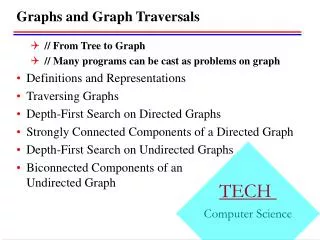
Chapter 12: Graphs Example A identified vertex A visited vertex A B C D unexplored edge discovery edge E F cross edge A A B C D B C D E F E F
Chapter 12: Graphs Example (cont.) A A B C D B C D E F E F A A B C D B C D E F E F
Chapter 12: Graphs Example (cont.) A A B C D B C D L2 E F E F A A B C D B C D E F E F
Analysis • Each vertex is enqued once and dequeued once : Θ(n) • Each adjacency list is traversed once: • Total: Θ(n+m)
BFS Tree • predecessor pointers after BFS is completed define an inverted tree • Reverse edges: BFS tree rooted at s • The edges of the BFS tree are called : discovery (tree) edges • Remaining graph edges are called: cross edges
BFS and shortest paths • Theorem: Let G=(V,E) be a directed or undirected graph, and suppose BFS is run on G starting from vertex s. During its execution BFS discovers every vertex v in V that is reachable from s. Let δ(s,v) denote the number of edges on the shortest path form s to v. Upon termination of BFS, d[v] = δ(s,v) for all v in V.
DFS • Start at a source vertex s • Search as far into the graph as possible and backtrack when there is no new vertices to discover • recursive
color[u] and pred[u] as before • color[u] • Undiscovered: white • Discovered but not finished processing: gray • Finished: black • pred[u] • Pointer to the vertex that first discovered u
Time stamps, • We store two time stamps: • d[u]: the time vertex u is first discovered (discovery time) • f[u]: the time we finish processing vertex u (finish time)
DFS(G) for each (u in V) do color[u] = white pred[u] = NIL time = 0 for each (u in V) do if (color[u] == white) DFS-VISIT(u) DFS-VISIT(u) //vertex u is just discovered color[u] = gray time = time +1 d[u] = time for each (v in Adj[u]) do //explore neighbor v if (color[v] == white) then //v is discovered by u pred[v] = u DFS-VISIT(v) color[u] = black // u is finished f[u] = time = time+ 1 DFS-VISIT invoked by each vertex exactly once. Θ(V+E)
A C B D E DFS Forest • Tree edges: inverse of pred[] pointers • Recursion tree, where the edge (u,v) arises when processing a vertex u, we call DFS-VISIT(v) Remaining graph edges are classified as: • Back edges: (u, v) where v is an ancestor of u in the DFS forest (self loops are back edges) • Forward edges: (u, v) where v is a proper descendent of u in the DFS forest • Cross edges: (u,v) where u and v are not ancestors or descendents of one another. s
If DFS run on an undirected graph • No difference between back and forward edges: all called back edges • No cross edges: can you see why?
Parenthesis Theorem • In any DFS of a graph G= (V,E), for any two vertices u and v, exactly one of the following three conditions holds: • The intervals [d[u],f[u]] and [d[v],f[v]] are entirely disjoint and neither u nor v is a descendent of the other in the DFS forest • The interval [d[u],f[u]] is contained within interval [d[v],f[v]] and u is a descendent of v in the DFS forest • The interval [d[v],f[v]] is contained within interval [d[u],f[u]] and v is a descendent of u in the DFS forest
How can we use DFS to determine whether a graph contains any cycles?