Download
1 / 48
480 likes | 633 Views
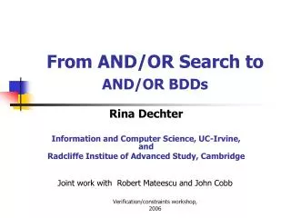
From AND/OR Search to AND/OR BDDs. Rina Dechter Information and Computer Science, UC-Irvine, and Radcliffe Institue of Advanced Study, Cambridge. Joint work with Robert Mateescu and John Cobb. A. B. B. A. C. C. C. C. B. B. D. D. D. D. D. D. D. D. E. E. G. G. E. E. E.

E N D
From AND/OR Search to AND/OR BDDs Rina Dechter Information and Computer Science, UC-Irvine, and Radcliffe Institue of Advanced Study, Cambridge Joint work with Robert Mateescu and John Cobb Verification/constraints workshop, 2006
A B B A C C C C B B D D D D D D D D E E G G E E E E E E F H 0 1 0 1 F F F G G H 0 1 Combining Decision Diagrams g = C*G +D*H f = A*E + B*F OBDD f * g =
A A C C B B B B D D D D AND E E E E G G G G F F H H 0 0 1 1 0 0 1 1 Combining AND/OR BDDs g = C*G +D*H f = A*E + B*F AOBDD f * g =
A B B A C C C C B B D D D D D D D D AND E E G G E E E E E E F H 0 1 0 1 F F F G G H 0 1 OBDDs vs AOBDD f * g = AOBDD OBDD
Outline • Background in Graphical models • AND/OR search trees and Graphs • Minimal AND/OR graphs • From AND/OR graphs to AOMDDs • Compilation of AOMDDs • AOMDDs and earlier BDDs
E A B red green red yellow green red green yellow yellow green yellow red A D B F G C Constraint Networks A Example: map coloring Variables - countries (A,B,C,etc.) Values - colors (red, green, blue) Constraints: Constraint graph A E D F B G C Semantics: set of all solutions Primary task: find a solution
Propositional Satisfiability = {(¬C),(A v B v C),(¬A v B v E), (¬B v C v D)}.
A F B C E D Graphical models • A graphical model (X,D,C): • X = {X1,…Xn} variables • D = {D1, … Dn} domains • C = {F1,…,Ft} functions(constraints, CPTS, cnfs) • Examples: • Constraint networks • Belief networks • Cost networks • Markov random fields • Influence diagrams • All these tasks are NP-hard • identify special cases • approximate
P(X) P(Y|X) P(Z|X) P(T|Y) P(R|Y) P(L|Z) P(M|Z) Tree-solving is easy CSP – consistency (projection-join) Belief updating (sum-prod) #CSP (sum-prod) MPE (max-prod) Trees are processed in linear time and memory
Transforming into a Tree • By Inference (thinking) • Transform into a single, equivalent tree of sub-problems • By Conditioning (guessing) • Transform into many tree-like sub-problems.
Inference and Treewidth ABC DGF G D A B BDEF F C EFH E M K H FHK L J Inference algorithm: Time: exp(tree-width) Space: exp(tree-width) HJ KLM treewidth = 4 - 1 = 3 treewidth = (maximum cluster size) - 1
H H H G G G N N N H H G G D D D N N F F F M M M D D A A A A J J J F F M M O O O J J E E E O O E E C C C P P P B B B C C P P B B K K K L L L K K L L B H H H G G G N N N D D D C F F M M F M J J J O O O E E E C C P P P K K L L K L Conditioning and Cycle cutset Cycle cutset = {A,B,C}
E M D Graph Coloring problem L C A B K H F G J A=yellow A=green E M E M D D L L C C B B K K H H F F G G J J Search over the Cutset • Inference may require too much memory • Condition (guessing) on some of the variables
E M D Graph Coloring problem L C A B K H F G J A=yellow A=green B=red B=blue B=green B=red B=blue B=yellow E E E E E E M M M M M M D D D D D D L L L L L L C C C C C C K K K K K K H H H H H H F F F F F F G G G G G G J J J J J J Search over the Cutset (cont) • Inference may require too much memory • Condition on some of the variables
ABC DGF G D A BDEF B F C EFH E M K H FHK L J KLM HJ A=yellow A=green B=blue B=green B=red B=blue E M D L C A E E E E M M M M D D D D L L L L B K C C C C H F K K K K G J H H H H F F F F G G G G J J J J Inference vs. Conditioning • By Inference (thinking) Exponential in treewidth Time and memory Variable-elimination Directional resolution Join-tree clustering • By Conditioning (guessing) Exponential in cycle-cutset Time-wise, linear memory Backtracking Branch and bound Depth-first search
Outline • Background in Graphical models • AND/OR searchtrees and Graphs • Minimal AND/OR graphs • From AND/OR graphs to AOMDDs • Compilation of AOMDDs • AOMDDs and earlier BDDs
A F B C E D A B E C D F Classic OR Search Space Ordering: A B E C D F 0 1 0 1 0 1 0 1 0 1 0 1 0 1 0 1 0 1 0 1 0 1 0 1 0 1 0 1 0 1 0 1 0 1 0 1 0 1 0 1 0 1 0 1 0 1 0 1 0 1 0 1 0 1 0 1 0 1 0 1 0 1 0 1 0 1 0 1 0 1 0 1 0 1 0 1 0 1 0 1 0 1 0 1 0 1 0 1 0 1 0 1 0 1 0 1 0 1 0 1 0 1 0 1 0 1 0 1 0 1 0 1 0 1 0 1 0 1 0 1 0 1 0 1 0 1
A A F F B B C C E E D D A B OR A E C AND 0 1 D F OR B B AND 0 0 1 1 OR E C E C E C E C AND 0 1 0 1 0 1 0 1 0 1 0 1 0 1 0 1 OR D F D F D F D F D F D F D F D F AND 0 1 0 1 0 1 0 1 0 1 0 1 0 1 0 1 0 1 0 1 0 1 0 1 0 1 0 1 0 1 0 1 AND/OR Search Space A F B C E D Primal graph DFS tree
A F B C E D A B A 0 1 E C B 0 1 0 1 D F A E 0 1 0 1 0 1 0 1 0 1 B C 0 1 0 1 0 1 0 1 0 1 0 1 0 1 0 1 0 1 0 1 E D 0 1 0 1 0 1 0 1 0 1 0 1 0 1 0 1 0 1 0 1 0 1 0 1 0 1 0 1 0 1 0 1 0 1 0 1 0 1 0 1 C F 0 1 0 1 0 1 0 1 0 1 0 1 0 1 0 1 0 1 0 1 0 1 0 1 0 1 0 1 0 1 0 1 0 1 0 1 0 1 0 1 0 1 0 1 0 1 0 1 0 1 0 1 0 1 0 1 0 1 0 1 0 1 0 1 0 1 0 1 0 1 0 1 0 1 0 1 0 1 0 1 D 0 1 0 1 0 1 0 1 0 1 0 1 0 1 0 1 0 1 0 1 0 1 0 1 0 1 0 1 0 1 0 1 F 0 1 0 1 0 1 0 1 0 1 0 1 0 1 0 1 0 1 0 1 0 1 0 1 0 1 0 1 0 1 0 1 0 1 0 1 0 1 0 1 0 1 0 1 0 1 0 1 0 1 0 1 0 1 0 1 0 1 0 1 0 1 0 1 AND/OR vs. OR OR A AND 0 1 AND/OR OR B B AND 0 0 1 1 OR E C E C E C E C AND 0 1 0 1 0 1 0 1 0 1 0 1 0 1 0 1 OR D F D F D F D F D F D F D F D F AND 0 1 0 1 0 1 0 1 0 1 0 1 0 1 0 1 0 1 0 1 0 1 0 1 0 1 0 1 0 1 0 1 AND/OR size: exp(4), OR size exp(6) 0 OR 1 1 1 0 1
A F B C E D A B A OR A 0 1 E C B 0 1 0 1 D F A A E 0 0 1 1 0 1 0 1 0 1 0 1 B B C 0 0 1 1 0 0 1 1 0 1 0 1 0 1 0 1 0 1 0 1 0 1 0 1 E E D 0 0 1 1 0 0 1 1 0 0 1 1 0 0 1 1 0 1 0 1 0 1 0 1 0 1 0 1 0 1 0 1 0 1 0 1 0 1 0 1 0 1 0 1 0 1 0 1 C C F 0 0 1 1 0 0 1 1 0 0 1 1 0 0 1 1 0 0 1 1 0 0 1 1 0 0 1 1 0 0 1 1 0 1 0 1 0 1 0 1 0 1 0 1 0 1 0 1 0 1 0 1 0 1 0 1 0 1 0 1 0 1 0 1 0 1 0 1 0 1 0 1 0 1 0 1 0 1 0 1 0 1 0 1 0 1 0 1 0 1 0 1 0 1 0 1 D D 0 0 1 1 0 0 1 1 0 0 1 1 0 0 1 1 0 0 1 1 0 0 1 1 0 0 1 1 0 0 1 1 0 0 1 1 0 0 1 1 0 0 1 1 0 0 1 1 0 0 1 1 0 0 1 1 0 0 1 1 0 0 1 1 F F 0 0 1 1 0 0 1 1 0 0 1 1 0 0 1 1 0 0 1 1 0 0 1 1 0 0 1 1 0 0 1 1 0 0 1 1 0 0 1 1 0 0 1 1 0 0 1 1 0 0 1 1 0 0 1 1 0 0 1 1 0 0 1 1 0 0 1 1 0 0 1 1 0 0 1 1 0 0 1 1 0 0 1 1 0 0 1 1 0 0 1 1 0 0 1 1 0 0 1 1 0 0 1 1 0 0 1 1 0 0 1 1 0 0 1 1 0 0 1 1 0 0 1 1 0 0 1 1 No-goods (A=1,B=1) (B=0,C=0) AND/OR vs. ORwith Constraints AND 0 1 AND/OR OR B B AND 0 0 1 1 OR E C E C E C E C AND 0 1 0 1 0 1 0 1 0 1 0 1 0 1 0 1 OR D F D F D F D F D F D F D F D F AND 0 1 0 1 0 1 0 1 0 1 0 1 0 1 0 1 0 1 0 1 0 1 0 1 0 1 0 1 0 1 0 1 OR
A F B C E D A B E C D F AND/OR vs. ORwith Constraints No-goods (A=1,B=1) (B=0,C=0 OR A AND 0 1 AND/OR OR B B AND 0 0 1 OR E C E C E C AND 0 1 1 0 1 1 0 1 0 1 OR D F D F D F D F AND 0 1 0 1 0 1 0 1 0 1 0 1 0 1 0 1 A A A 0 0 0 1 1 1 OR B B B 0 0 0 1 1 1 0 0 0 E E E 0 0 0 1 1 1 0 0 0 1 1 1 0 0 0 1 1 1 C C C 1 1 1 1 1 1 0 0 0 1 1 1 0 0 0 1 1 1 1 1 1 1 1 1 D D D 0 0 0 1 1 1 0 0 0 1 1 1 0 0 0 1 1 1 0 0 0 1 1 1 0 0 0 1 1 1 0 0 0 1 1 1 0 0 0 1 1 1 0 0 0 1 1 1 F F F 0 0 0 1 1 1 0 0 0 1 1 1 0 0 0 1 1 1 0 0 0 1 1 1 0 0 0 1 1 1 0 0 0 1 1 1 0 0 0 1 1 1 0 0 0 1 1 1 0 0 0 1 1 1 0 0 0 1 1 1 0 0 0 1 1 1 0 0 0 1 1 1 0 0 0 1 1 1 0 0 0 1 1 1 0 0 0 1 1 1 0 0 0 1 1 1
A F B C solution E D OR A 11 AND 6 5 1 B OR B 5 6 E C AND 1 0 1 1 4 2 OR E C E C E C 1 1 4 2 1 1 D F AND 0 0 1 0 1 0 1 0 1 0 1 0 1 1 2 1 2 1 1 0 1 0 0 1 OR D F D F D F D F D F D F 1 1 1 0 2 1 2 1 1 1 1 1 AND 0 1 0 1 0 1 0 1 0 1 0 1 0 1 0 1 0 1 0 1 0 1 0 1 1 0 1 0 0 1 0 0 1 1 1 0 1 1 1 0 1 0 1 0 0 1 1 0 DFS algorithm (#CSP example) A 0 B 4 0 OR node: Marginalization operator (summation) E C 2 2 AND node: Combination operator (product) 0 2 0 1 0 1 1 1 D F D F 2 1 2 0 0 1 0 1 0 1 0 1 1 1 1 0 1 1 0 0 Value of node = number of solutions below it
Pseudo-Trees (Freuder 85, Bayardo 95,Bodlaender and Gilbert, 91) 1 4 1 6 2 3 2 7 5 3 m <= w* log n (a) Graph 4 7 1 1 2 7 5 3 5 3 5 4 2 7 6 6 4 6 (b) DFS tree depth=3 (c) pseudo- tree depth=2 (d) Chain depth=6
Tasks and value of nodes • V( n) is the value of the tree T(n) for the task: • Consistency: v(n) is 0 if T(n) inconsistent, 1 othewise. • Counting: v(n) is number of solutions in T(n) • Optimization: v(n) is the optimal solution in T(n) • Belief updating: v(n), probability of evidence in T(n). • Partition function: v(n) is the total probability in T(n). • Goal: compute the value of the root node recursively using dfs search of the AND/OR tree. • AND/OR search tree and algorithms are ([Freuder & Quinn85], [Collin, Dechter & Katz91], [Bayardo & Miranker95],[Darwiche 2001], [Bacchus et. Al, 2003]) • Space:O(n) • Time:O(exp(m)), where m is the depth of the pseudo-tree • Time:O(exp(w* log n)) • BFS is time and spaceO(exp(w* log n)
0 1 0 1 0 1 0 1 0 1 0 1 0 1 0 1 0 1 0 1 0 1 0 1 0 1 0 1 0 1 0 1 J J J J G G J J G G J J J J G G J J G G G G J J G G J J G G G G 0 1 0 1 0 1 0 1 0 1 0 1 0 1 0 1 0 1 0 1 0 1 0 1 0 1 0 1 0 1 0 1 0 1 0 1 0 1 0 1 0 1 0 1 0 1 0 1 0 1 0 1 0 1 0 1 0 1 0 1 0 1 0 1 H H H H K K K K H H H H K K K K H H H H K K K K H H H H K K K K H H H H K K K K H H H H K K K K H H H H K K K K H H H H K K K K 0 1 0 1 0 1 0 1 0 1 0 1 0 1 0 1 0 1 0 1 0 1 0 1 0 1 0 1 0 1 0 1 0 1 0 1 0 1 0 1 0 1 0 1 0 1 0 1 0 1 0 1 0 1 0 1 0 1 0 1 0 1 0 1 0 1 0 1 0 1 0 1 0 1 0 1 0 1 0 1 0 1 0 1 0 1 0 1 0 1 0 1 0 1 0 1 0 1 0 1 0 1 0 1 0 1 0 1 0 1 0 1 0 1 0 1 0 1 0 1 0 1 0 1 0 1 0 1 A J A From AND/OR Tree F B B C K E C E D D F G J G H OR A H K AND 0 1 OR B B AND 0 0 1 1 OR E C E C E C E C AND 0 1 0 1 0 1 0 1 0 1 0 1 0 1 0 1 OR D F D F D F D F D F D F D F D F AND OR AND OR AND
A J A To an AND/ORGraph F B B C K E C E D D F G J G H OR A H K AND 0 1 OR B B AND 0 0 1 1 OR E C E C E C E C AND 0 1 0 1 0 1 0 1 0 1 0 1 0 1 0 1 OR D F D F D F D F D F D F D F D F AND 0 1 0 1 OR J J G G AND 0 1 0 1 0 1 0 1 OR H H H H K K K K AND 0 1 0 1 0 1 0 1 0 1 0 1 0 1 0 1
AND/OR Search Graphs • Any two nodes that root identical subtrees/subgraphs (are unifiable) can be merged • Minimal AND/OR search graph:of R relative to tree T is theclosure under merge of the AND/OR search tree of R relative to T, where inconsistent subtrees are pruned. • Canonicity: The minimal AND/OR graph relative to T is unique for all constraints equivalent to R.
A J A F B B C K E C E D D F G J G H H K Context based caching • Caching is possible when context is the same • context = parent-separator set in induced pseudo-graph = current variable + ancestors connected to subtree below context(B) = {A, B} context(C) = {A,B,C} context(D) = {D} context(F) = {F}
0 1 0 1 0 1 0 1 0 1 0 1 0 1 0 1 0 1 0 1 0 1 0 1 0 1 0 1 0 1 0 1 J J J J G G J J G G J J J J G G J J G G G G J J G G J J G G G G 0 1 0 1 0 1 0 1 0 1 0 1 0 1 0 1 0 1 0 1 0 1 0 1 0 1 0 1 0 1 0 1 0 1 0 1 0 1 0 1 0 1 0 1 0 1 0 1 0 1 0 1 0 1 0 1 0 1 0 1 0 1 0 1 H H H H K K K K H H H H K K K K H H H H K K K K H H H H K K K K H H H H K K K K H H H H K K K K H H H H K K K K H H H H K K K K 0 1 0 1 0 1 0 1 0 1 0 1 0 1 0 1 0 1 0 1 0 1 0 1 0 1 0 1 0 1 0 1 0 1 0 1 0 1 0 1 0 1 0 1 0 1 0 1 0 1 0 1 0 1 0 1 0 1 0 1 0 1 0 1 0 1 0 1 0 1 0 1 0 1 0 1 0 1 0 1 0 1 0 1 0 1 0 1 0 1 0 1 0 1 0 1 0 1 0 1 0 1 0 1 0 1 0 1 0 1 0 1 0 1 0 1 0 1 0 1 0 1 0 1 0 1 0 1 A J A Caching F B B C K E C E D D F G J G H context(B) = {A, B} context(C) = {A,B,C} context(D) = {D} context(F) = {F} OR A H K AND 0 1 OR B B AND 0 0 1 1 OR E C E C E C E C AND 0 1 0 1 0 1 0 1 0 1 0 1 0 1 0 1 OR D F D F D F D F D F D F D F D F AND OR AND OR AND
A J A Caching F B B C K E C E D D F context(D)={D} context(F)={F} G J G H OR A H K AND 0 1 OR B B AND 0 0 1 1 OR E C E C E C E C AND 0 1 0 1 0 1 0 1 0 1 0 1 0 1 0 1 OR D F D F D F D F D F D F D F D F AND 0 1 0 1 OR J J G G AND 0 1 0 1 0 1 0 1 OR H H H H K K K K AND 0 1 0 1 0 1 0 1 0 1 0 1 0 1 0 1
A 0 1 B 0 1 0 1 C C A F 0 1 0 1 0 1 0 1 D 0 1 0 1 0 1 0 1 D B E E 0 1 0 1 F 0 1 OR OR A A A AND AND 0 1 0 1 0 1 B OR OR 0 1 0 1 B B B B C AND AND 0 1 0 1 0 1 0 1 1 1 0 0 1 1 0 0 D OR C C C C OR E 0 1 0 1 0 1 0 1 0 1 0 1 0 1 0 1 E C E E C C C E E E E E AND AND 0 1 0 1 0 1 0 1 0 1 0 1 0 1 0 1 0 1 0 1 0 1 0 1 0 1 0 1 0 1 0 1 0 1 0 1 0 1 0 1 0 1 0 1 0 1 0 1 0 1 0 1 0 1 0 1 F OR D D D D OR 0 1 0 1 0 1 0 1 0 1 0 1 0 1 0 1 0 1 0 1 0 1 0 1 0 1 0 1 0 1 0 1 0 1 0 1 0 1 0 1 0 1 0 1 0 1 0 1 0 1 0 1 0 1 0 1 0 1 0 1 0 1 0 1 F F F F D D D D D D D D F F F F F F F F AND AND 0 1 0 1 0 1 0 1 0 1 0 1 0 1 0 1 0 1 0 1 0 1 0 1 0 1 0 1 0 1 0 1 0 1 0 1 All Four Search Spaces Full OR search tree 126 nodes Context minimal OR search graph 28 nodes Context minimal AND/OR search graph 18 AND nodes Full AND/OR search tree 54 AND nodes
Properties of minimal AND/OR graphs Complexity: • MinimalAND/OR R relative to pseudo-tree T is O(exp(w*)) where w* is the tree-width of R along T. • Minimal OR search graph is O(exp(pw*)) where pw* is path-width • w* ≤ pw*, pw* ≤ w*log n Canonicity: • The minimal AND/OR search graph is unique (canonical) for all equivalent formulas (Boolean or Constraints), consistent with its pseudo tree.
Searching AND/OR Graphs • AO(j): searches depth-first, cache i-context • j = the max size of a cache table (i.e. number of variables in a context) i=0 i=w* j Space: O(exp w*) Time: O(exp w*) Space: O(n) Time: O(exp(w* log n)) Space: O(exp(j) ) Time: O(exp(m_j+j )
C A F D B E A 5 7 0 1 B B 7 5 6 5 6 4 0 1 0 1 C C C C 4 3 4 E E E 4 E 2 0 5 2 0 1 0 1 D D D D Context-Based Caching context(A) = {A} context(B) = {B,A} context(C) = {C,B} context(D) = {D} context(E) = {E,A} context(F) = {F} A B Primal graph C E D F Cache Table (C) Space: O(exp(2))
Outline • Background in Graphical models • AND/OR search trees and Graphs • Minimal AND/OR graphs • From AND/OR search graphs to AOMDDs • Compilation of AOMDDs • AOMDDs and earlier BDDs
A 0 1 B B 0 1 0 1 C C C C 0 1 0 1 0 1 0 1 Full AND/OR search tree A A 0 1 0 1 A 0 1 B B B 1 B B 1 0 1 1 0 1 C C C C 1 C 1 1 1 An OBDD 1 Backtrack free AND/OR search tree OR Search Graphs vs OBDDs A B C redundant Minimal AND/OR search graph
A B A B A D C 0 1 0 0 1 1 AND/OR Search Graphs; AOBDDs F(A,B,C,D)= (0,1,1,1), (1,0,1,0), (1,1,1,0) AOBDD(F) B redundancy B 1 1 D C D D C 1 1 0 D 1 1 0
A B A B A D C 0 1 0 0 1 1 AND/OR Search Graphs; AOBDDs F(A,B,C,D)= (0,1,1,1), (1,0,1,0), (1,1,1,0) AOBDD(F) B redundancy B 1 1 D C D D C 1 1 0 D 1 1 0
A B D C D B A A D C 0 0 0 0 0 1 1 1 1 1 0 1 B 1 C D D 1 1 0 0 1 AOBDD Conventions Point dead-ends to terminal 0 Point goods to terminal 1
A B A D C B D A D C 0 0 0 0 0 1 1 1 1 1 0 1 B 1 C D D 1 1 0 0 1 AOBDD Conventions Introduce Meta-nodes
B D D D C D B A A 0 0 0 0 0 0 0 0 0 1 1 1 1 1 1 1 1 1 A 0 1 B 0 1 C 0 1 0 1 0 1 0 1 Combining AOBDD (apply) A A A B B B C D D C = *
A A D G B C B F C F A m7 E A H D E G H B primal graph pseudo tree B C F 0 1 m6 m6 m3 0 1 m3 D E G H A A B F 0 1 0 1 B C F C9 C5 0 1 0 1 0 1 m2 C m4 m1 m5 0 1 m1 m5 m4 G H m2 D E A A A C C B E C D B B C D D A D G C B B E E E F G G A A B F C C B C H A F A G H H F F G F H F F C C B H B G H F C D F B G A B A A D 0 1 0 1 0 1 0 1 0 1 0 1 F E H D 0 0 0 0 0 0 0 0 0 0 0 0 0 0 0 0 0 0 0 0 0 0 0 0 0 0 0 0 0 0 0 0 0 0 0 0 0 0 0 0 0 0 0 0 0 0 0 0 0 0 0 0 0 0 0 0 0 0 0 0 1 1 1 1 1 1 1 1 1 1 1 1 1 1 1 1 1 1 1 1 1 1 1 1 1 1 1 1 1 1 1 1 1 1 1 1 1 1 1 1 1 1 1 1 1 1 1 1 1 1 1 1 1 1 1 1 1 1 1 1 C8 E G D C1 C4 C6 C7 C2 F C3 0 1 H G Example: (f+h) * (a+!h) * (a#b#g) * (f+g) * (b+f) * (a+e) * (c+e) * (c#d) * (b+c) m7
A m7 B C F 0 1 m6 A 0 1 m3 D E G H 0 1 m7 B E G G F B H D C B F G G F B D F C H F A F A C C D C E C D H C A B F H F C B B 0 0 0 0 0 0 0 0 0 0 0 0 0 0 0 0 0 0 0 0 0 1 1 1 1 1 1 1 1 1 1 1 1 1 1 1 1 1 1 1 1 1 0 0 0 0 0 0 0 0 0 0 0 0 0 0 0 0 0 0 1 1 1 1 1 1 1 1 1 1 1 1 1 1 1 1 1 1 Example (continued)
D G C B F A E A H B primal graph C F D E G H 0 1 C G F F C B G F H A B D C E H F D C 0 0 0 0 0 0 0 0 0 0 0 0 0 0 0 0 0 0 1 1 1 1 1 1 1 1 1 1 1 1 1 1 1 1 1 1 AOBDD vs. OBDD A B B C C C C D D D D D D E E E F F F F G G G G G A H H B C 1 0 D AOBDD 18 nonterminals 47 arcs OBDD 27 nonterminals 54 arcs E F G H
Complexity • Complexity of apply: Complexity of apply is bounded quadratically by the product of input AOBDDs restricted to each branch in the output pseudo-tree. • Complexity of VE-AOBDD: is exponential in the tree-width along the pseudo-tree.
AOMDDs and tree-BDDs • Tree-BDDs (McMillan1994) are : • AND/OR BDDS are
Related work • Related work in Search • Backjumping + learning (Freuder 1988,Dechter 1990,Bayardo and Mirankar 1996) • Recursive-conditioning (Darwiche 2001) • Value elimination (Bacchus et. Al. 2003) • Search over tree-decompositions (Trrioux et. Al. 2002) • Related to compilation schemes: • Minimal AND/OR – related to tree-OBDDs (McMillan 94), • d-DNNF (Darwiche et. Al. 2002) • Case-factor diagrams (Mcallester, Collins, Pereira, 2005) • Tutorial references: • Dechter, Constraint processing, Morgan Kauffman, 2003 • Dechter, Tractable Structures of Constraint Satisfaction problems, In Handbook of constraint solving, forthcoming.
Conclusion • AND/OR search should always be used. • AND/OR BDDs are superior to OBDDs. • A search algorithm with good and no-good learning generates an OBDD or an AND/OR Bdds. • Dynamic variable ordering can be incorporated • With caching, AND/OR search is similar to inference (variable-elimination) • The real tradeoff should be rephrased: • Time vs space rather than search vs inference, or search vs model-checking. • Search methods are more sensitive to this tradeoff.