Bayes Factors
490 likes | 612 Views
Learn about hypothesis testing, Bayes Theorem, Bayesian model selection, and Bayes Factors. Understand how to compute evidence for alternative and null hypotheses using Bayes Factor. Explore practical applications in psychological science.

Bayes Factors
E N D
Presentation Transcript
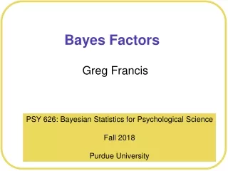
Bayes Factors Greg Francis PSY 626: Bayesian Statistics for Psychological Science Fall 2018 Purdue University
Hypothesis testing • Suppose the null is true and check to see if a rare event has occurred • e.g., does our random sample produce a t value that is in the tails of the null sampling distribution? • If a rare event occurred, reject the null hypothesis
Hypothesis testing • But what is the alternative? • Typically: “anything goes” • But that seems kind of unreasonable • Maybe the “rare event” would be even less common if the null were not true!
Bayes Theorem • Conditional probabilities
Ratio • Ratio of posteriors conveniently cancels out P(D) Posterior odds Bayes Factor Prior odds
Bayesian Model Selection • It’s not really about hypotheses, but hypotheses suggest models • The Bayes Factor is often presented as BF12 • You could also compute BF21 Posterior odds Bayes Factor Prior odds
Bayes Factor Evidence for the alternative hypothesis (or the null) is computed with the Bayes Factor (BF) • BF>1 indicates that the data is evidence for the alternative, compared to the null • BF<1 indicates that the data is evidence for the null, compared to the alternative
Bayes Factor When BF10 = 2, the data are twice as likely under H1 as under H0. When BF01 = 2, the data are twice as likely under H0 as under H1. These interpretations do not require you to believe that one model is better than the other You can still have priors that favor one model, regardless of the Bayes Factor You would want to make important decisions based on the posterior Still, if you consider both models to be plausible, then the priors should not be so different from each other
Rules of thumb Evidence for the alternative hypothesis (or the null) is computed with the Bayes Factor (BF)
Similar to AIC • For a two-sample t-test, the null hypothesis (reduced model) is that a score from group s (1 or 2) is defined as • With the same mean for each group s X12 X11 X22 X21
AIC • For a two-sample t-test, the alternative hypothesis (full model) is that a score from group s (1 or 2) is defined as • With different means for each group s X12 X11 X22 X21
AIC • AIC and its variants are a way of comparing model structures • One mean or two means? • Always uses maximum likelihood estimates of the parameters • Bayesian approaches identify a posterior distribution of parameter values • We should use that information!
Models of what? • We have been building models of trial-level scores # Model without intercept (more natural) model2 = brm(Leniency ~ 0+SmileType, data = SLdata, iter = 2000, warmup = 200, chains = 3) print(summary(model2)) GrandSE = 10 stanvars <-stanvar(GrandMean, name='GrandMean') + stanvar(GrandSE, name='GrandSE') prs <- c(prior(normal(GrandMean, GrandSE), class = "b") ) model6 = brm(CorrectResponses ~ 0 + Dosage + (1 |SubjectID), data = ATdata, iter = 2000, warmup = 200, chains = 3, thin = 2, prior = prs, stanvars=stanvars ) print(summary(model6))
Models of what? • We have been building models of trial-level scores • That is not the only option • In traditional hypothesis testing, we care more about effect sizes than about individual scores • Signal-to-noise ratio • Of course, the effect size is derived from the individual scores • In many cases, it is enough to just model the effect size itself rather than the individual scores • Cohen’s d • t-statistic • p-value • Correlation r • “Sufficient” statistic
Models of means • It’s not really going to be practical, but let’s consider a case where we assume that the population variance is known (and equals 1) and we want to compare null and alternative hypotheses of fixed values
Models of means • The likelihood of any given observed mean value is derived from the sampling distribution • Suppose n=100 (one sample)
Models of means • The likelihood of any given observed mean value is derived from the sampling distribution • Suppose n=100 (one sample) Suppose we observe Data are more likely under null than under alternative
Models of means • The likelihood of any given observed mean value is derived from the sampling distribution • Suppose n=100 (one sample) Suppose we observe Data are more likely under alternative than under null
Models of means • The likelihood of any given observed mean value is derived from the sampling distribution • Suppose n=100 (one sample) Suppose we observe Data are more likely under alternative than under null
Bayes Factor • The ratio of likelihood for the data under the null compared to the alternative • Or the other way around Suppose we observe Data are more likely under alternative than under null
Decision depends on alternative • The likelihood of any given observed mean value is derived from the sampling distribution • Suppose n=100 (one sample) Suppose we observe Data are more likely under null than under alternative
Decision depends on alternative • The likelihood of any given observed mean value is derived from the sampling distribution • Suppose n=100 (one sample)
Decision depends on alternative • The likelihood of any given observed mean value is derived from the sampling distribution • Suppose n=100 (one sample)
Decision depends on alternative For a fixed sample mean, evidence for the alternative only happens for alternative population mean values of a given range For big alternative values, the observed sample mean is less likely than for a null population value • The sample mean may beunlikely for both models • Rouder et al. (2009) Evidence for null Evidence for alternative Mean of alternative
Models of means • Typically, we do not hypothesize a specific value for the alternative, but a range of plausible values
Likelihoods • For the null, we compute likelihood in the same way • Suppose n=100 (one sample)
Likelihoods • For the alternative, we have to consider each possible value of mu, compute the likelihood of the sample mean for that value, and then average across all possible values • Suppose n=100 (one sample)
Likelihoods • For the alternative, we have to consider each possible value of mu, compute the likelihood of the sample mean for that value, and then average across all possible values • Suppose n=100 (one sample)
Likelihoods • For the alternative, we have to consider each possible value of mu, compute the likelihood of the sample mean for that value, and then average across all possible values • Suppose n=100 (one sample)
Likelihoods • For the alternative, we have to consider each possible value of mu, compute the likelihood of the sample mean for that value, and then average across all possible values • Suppose n=100 (one sample)
Average Likelihood • For the alternative, we have to consider each possible value of mu, compute the likelihood of the sample mean for that value, and then average across all possible values • Suppose n=100 (one sample) Prior for value of mu Likelihood for given value of mu (from sampling distribution)
Bayes Factor • Ratio of the likelihood for the null compared to the (average) likelihood for the alternative P(D | H1)
Uncertainty • The prior standard deviation for mu establishes a range of plausible values for mu More flexible Less flexible
Uncertainty 0.15 0.15 • With a very narrow prior, you may not fit the data More flexible Less flexible
Uncertainty 0.15 0.15 • With a very broad prior, you will fit well for some values of mu and poorly for other values of mu More flexible Less flexible
Uncertainty 0.15 0.15 • Uncertainty in the prior functions similar to the penalty for parameters in AIC More flexible Less flexible
Penalty • Averaging acts like a penalty for extra parameters • Rouder et al. (2009) Evidence for null Evidence for alternative Width of alternative prior
Models of effect size • Consider the case of two-sample t-test • We often care about the standardized effect size • Which we can estimate from data as:
Models of effect size • If we were doing traditional hypothesis testing, we would compare a null model: • Against an alternative: • Equivalent statements can be made using the standardized effect size • As long as the standard deviation is not zero
Priors on effect size • For the null, the prior is (again) a spike at zero
JZS Priors on effect size • For the alternative, a good choice is a Cauchy distribution (t-distribution with df=1) Rouder et al. (2009) Jeffreys, Zellner, Siow
JZS Priors on effect size • It is a good choice because the integration for the alternative hypothesis can be done numerically • t is the t-value you use in a hypothesis test (from the data) • v is the “degrees of freedom” (from the data) • This might not look easy, but it is simple to calculate with a computer
Variations of JZS Priors • Scale parameter “r” • Bigger values make for a broader prior • More flexibility! • More penalty!
Variations of JZS Priors • Medium r= 1 • Wide r= sqrt(2)/2 • Ultrawide r=sqrt(2)
How do we use it? • Super easy • Rouder’s web site: • http://pcl.missouri.edu/bayesfactor • In R • library(BayesFactor)
How do we use it? • library(BayesFactor) • ttest.tstat(t=2.2, n1=15, n2=15, simple=TRUE) • B10 • 1.993006
What does it mean? • Guidelines BFEvidence 1 – 3 Anecdotal 3 – 10 Substantial 10 – 30 Strong 30 – 100 Very strong >100 Decisive
Conclusions • JZS Bayes Factors • Easy to calculate • Pretty easy to understand results • A bit arbitrary for setting up • Why not other priors? • How to pick scale factor? • Criteria for interpretation are arbitrary • Fairly painless introduction to Bayesian methods