Download
1 / 41
891 likes | 3.02k Views
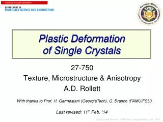
Plastic Deformation of Single Crystals. 27-750 Texture, Microstructure & Anisotropy A.D. Rollett. With thanks to Prof. H . Garmestani ( GeorgiaTech ), G . Branco (FAMU/FSU) . Last revised: 11 th Feb. ‘14. Objective.

E N D
Plastic Deformation of Single Crystals 27-750 Texture, Microstructure & Anisotropy A.D. Rollett With thanks to Prof. H. Garmestani (GeorgiaTech), G. Branco (FAMU/FSU) Last revised:11thFeb. ‘14
Objective • The objective of this lecture is to explain how single crystals deform plastically. • Subsidiary objectives include: • Schmid Law • Critical Resolved Shear Stress • Lattice reorientation during plastic deformation • Note that this development assumes that we load each crystal under stress boundary conditions. That is, we impose a stress and look for a resulting strain (rate).
Why is the Schmid factor useful? • The Schmid factor is a good predictor of which slip or twinning system will be active, especially for small plastic strains (< 5 %). • It has been used to analyze the plasticity of ordered intermetallics, especially Ni3Al and NiAl. • It has been used to analyze twinning in hexagonal metals, which is an essential deformation mechanism. • Some EBSD software packages will let you produce maps of Schmid factor. • Schmid factor has proven useful to visualize localization of plastic flow as a precursor to fatigue crack formation. • Try searching with “Schmid factor” (include the quotation marks).
Bibliography • U.F. Kocks, C. Tomé, H.-R. Wenk, Eds. (1998). Texture and Anisotropy, Cambridge University Press, Cambridge, UK: Chapter 8, Kinematics and Kinetics of Plasticity. • C.N. Reid (1973). Deformation Geometry for Materials Scientists. Oxford, UK, ISBN: 1483127249, Pergamon. • Khan and Huang (1999), Continuum Theory of Plasticity, ISBN: 0-471-31043-3, Wiley. • W. Hosford, (1993), The Mechanics of Crystals and Textured Polycrystals, Oxford Univ. Press. • G.E. Dieter (1986), Mechanical Metallurgy, ISBN: 0071004068, McGraw-Hill. • J.F. Nye (1957). Physical Properties of Crystals. Oxford, Clarendon Press. • T. Courtney, Mechanical Behavior of Materials, McGraw-Hill, 0-07-013265-8, 620.11292 C86M.
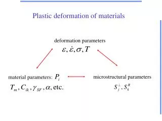
Notation • Strain (tensor), local: Elocal; global: Eglobal • Slip direction (unit vector): b (or m) • Slip plane (unit vector) normal: n(or s) • Stress (tensor): s • Shear stress (scalar, usually on a slip system): t • Angle between tensile axis and slip direction: • Angle between tensile axis and slip plane normal: • Schmid factor (scalar): m • Slip system geometry matrix (3x3): m • Taylor factor (scalar): M • Shear strain (scalar, usually on a slip system): g • Stress deviator (tensor): S • Rate sensitivity exponent: n • Slip system index: s(or ) • Set of Reference Axes: Oxi
Historical Development Physics of single-crystal plasticity • Established by Ewing and Rosenhaim(1900), Polanyi(1922), Taylor and others(1923/25/34/38), Schimd(1924), Bragg(1933) Mathematical representation • Initially proposed by Taylor in 1938, followed by Bishop & Hill (1951) • Further developments by Hill(1966), Kocks (1970), Hill and Rice(1972) , Asaro and Rice(1977), Hill and Havner(1983)
Physics of Slip Experimental technique Uniaxial Tension or Compression Experimental measurements showed that: • At room temperature the major source for plastic deformation is the dislocation motion through the crystal lattice • Dislocation motion occurs on fixed crystal planes (“slip planes”) in fixed crystallographic directions (corresponding to the Burgers vector of the dislocation that carries the slip) • The crystal structure of metals is not altered by the plastic flow • Volume changes during plastic flow are negligible, which means that the pressure (or, mean stress) does not contribute to plasticity
Shear Stress – Shear Strain Curves • A typical flow curve (stress-strain) for a single crystal shows three stages of work hardening: • Stage I = “easy glide” with low hardening rates ~µ/10000; - Stage II with high, constant (linear) hardening rate ~µ/200, nearly independent of temperature or strain rate; - Stage III with decreasing hardening rate and very sensitive to temperature and strain rate. Dynamic recovery operates; • Stage IV (not shown) with low hardening rates ~µ/10000. • Hardening behavior will be discussed in another lecture.
Burgers vector: b [Reid] Screw position:line direction//b A dislocation is a line defect in the crystal lattice. The defect has a definite magnitude and direction determined by the closure failure in the lattice found by performing a circuit around the dislocation line; this vector is known as the Burgers vector of the dislocation. It is everywhere the same regardless of the line direction of the dislocation. Dislocations act as carriers of strain in a crystal because they are able to change position by purely local exchange in atom positions (conservative motion) without any long range atom motion (i.e. no mass transport required). Edge position:line directionb
Slip steps Slip steps (where dislocations exitfrom the crystal) on the surface of compressed single crystal of Nb. [Reid]
Dislocation glide • The effect of dislocation motion in a crystal: passage causes one half of the crystal to be displaced relative to the other. This is a shear displacement, giving rise to a shear strain. [Dieter]
Single Crystal Deformation • To make the connection between dislocation behavior and yield strength as measured in tension, consider the deformation of a single crystal. • Given an orientation for single slip, i.e. the resolved shear stress reaches the critical value on one system ahead of all others, then one obtains a “pack-of-cards” straining. [Dieter]
Resolved Shear Stress = n • Geometry of slip: how big an applied stress is required for slip? • To obtain the resolved shearstress based on an applied tensilestress, P, take the component ofthe stress along the slip directionwhich is given by Fcosl, and divide by the area over which the (shear)force is applied, A/cosf. Note that the two angles are not complementary unless the slip direction, slip plane normal and tensile direction happen to be co-planar.t = (F/A) coslcosf = scoslcosf = s * m = b In tensor (index) form: = biij nj Schmid factor := m
Schmid’s Law Schmid postulated that: • Initial yield stress varies from sample to sample depending on, among several factors, the position of the crystal lattice relative to the loading axis. • It is the shear stress resolved along the slip direction on the slip plane that initiates plastic deformation. • Yield will begin on a slip system when the shear stress on this system first reaches a critical value (critical resolved shear stress, crss), independent of the tensile stress or any other normal stress on the lattice plane. E. Schmid & W. Boas (1950), Plasticity of Crystals, Hughes & Co., London.
Schmid’s Law Resolved Shear Stress
Critical Resolved Shear Stress • The experimental evidence of Schmid’s Law is that there is a critical resolved shear stress. This is verified by measuring the yield stress of single crystals as a function of orientation. The example below is for Mg which is hexagonal and slips most readily on the basal plane (all other tcrss are much larger). “Soft orientation”,with slip plane at45°to tensile axis s = t/coslcosf Exercise:draw a series of diagrams that illustrate where the tensile axis points in relation to the basal plane normal for different points along this curve “Hard orientation”,with slip plane at~90°to tensile axis
CalculationofResolvedShear Stress Using Schmid’s law
Rotation of the Crystal Lattice The slip direction rotates towards the tensile axis [Khan]
FCC Geometry of Slip Systems In fcc crystals, the slip systems are combinations of <110> slip directions (the Burgers vectors) and {111} slip planes. [Reid]
The combination of slip plane {a,b,c,d} and slip direction {1,2,3} that operates within each unit triangle is shown in the figure Slip Systems in fcc materials For FCC materials there are 12 slip systems (with + and - shear directions: Four {111} planes, each with three <011> directions: the letter denotes the plane, and the subscript number denotes the direction (in that plane). [Khan] Note correction to system b2
Geometry of Single Slip • For tensile stress applied in the [100]-[110]-[111] unit triangle, the most highly stressed slip system (highest Schmid factor) has a (11-1) slip plane and a [101] slip direction (the indices of both plane and direction are the negative of those shown on the previous page). • Caution: this diagram places [100] in the center, not [001]. [Hosford]
Schmid factors [Hosford] • The Schmid factors, m, vary markedly within the unit triangle (a). One can also (b) locate the position of the maximum (=0.5) as being equidistant between the slip plane and slip direction. (a) (b)
Names of Slip Systems • In addition to the primary slip system in a given triangle, there are systems with smaller resolved shear stresses. Particular names are given to some of these. For example the system that shares the same Burgers vector allows for cross-slip of screws and so is known as the cross slip system. The system in the triangle across the [100]-[111] boundary is the conjugate slip system. [Hosford]
Rotation of the Crystal Lattice in Tensile Test of an fcc Single Crystal [Hosford] The tensile axis rotates in tension towards the [100]-[111] line. If the tensile axis is in the conjugate triangle, then it rotates to the same line so there is convergence on this symmetry line. Once on the line, the tensile axis will rotate towards [211] which is a stable orientation. Note: the behavior in multiple slip is similar but there are significant differences in terms of the way in which the lattice re-orients relative to the tensile axis.
Rotation of the Crystal Lattice in Compression Test of an fcc Single Crystal The slip plane normal rotates towards the compression axis [Khan]
Useful Equations • Following the notation in Reid: n:= slip plane normal (unit vector); b:= slip direction (unit vector). • To find a new direction, D, based on an initial direction, d, after slip, use (and remember that crystal directions do not change): • To find a new plane normal, P, based on an initial plane normal, p, after slip, use the following: [Reid]
Taylor rate-sensitive model • We will find out later that the classical Schmid Law picture of elastic-perfectly plastic behavior is not sufficient. • In fact, there is a smooth transition from elastic to plastic behavior that can be described by a power-law behavior. • The shear strain rate on each slip system is given by the following (for a specified stress state), where* mij = binj, or m=b⊗n: * “m” is a slip tensor, formed as the outer product of the slip direction and slip plane normal
Schmid Law Calculations • To solve problems using the Schmid Law, use this pseudo-code: • Check that single slip is the appropriate model to use (as opposed to, say, multiple slip and the Taylor model); • Make a list of all 12 slip systems with slip plane normals (as unit vectors) and slip directions (as unit vectors that are perpendicular to their associated slip planes; check orthogonality by computing dot products); • Convert whatever information you have on the orientation of the single crystal into an orientation matrix, g; • Apply the inverse of the orientation to all planes and directions so that they are in specimen coordinates; • If the tensile stress is applied along the z-axis, for example, compute the Schmid factor as the product of the third components of the transformed plane and direction; • Inspect the list of absolute values of the Schmid factors: the slip system with the largest absolute value is the one that will begin to slip before the others; • Alternatively (for a general multi-axial state of stress), compute the following quantity, which resolves/projects the stress, , onto the kth slip system:
Hexagonal Metals • For typical hexagonal metals, the primary systems are:Basal slip {0001}<1-210>Prismatic slip {10-10}<1-210>Pyramidal twins {10-11}<1-210> • At room temperature and below for Zr, the systems are:Prismatic slip {10-10}<1-210>Tension twins {10-12}<10-11>, and {11-21}<-1-126>Compression twin {11-22}<-1-123>Also secondary pyramidal slip may play a limited role at RT: {10-11}<-2113>, or {11-21}<-2113>
Summary • The Schmid Law is well established for the dependence of onset of plastic slip as well as the geometry of slip. • Cubic metals have a limited set of slip systems: {111}<110> for fcc, and {110}<111> for bcc (neglecting pencil glide for now). • Hexagonal metals have a larger range of slip systems (see previous slide).
Basal (0002) Prism (0 -1 1 0) (2 -1 -1 0) Pyramidal (1 0 -1 1) Pyramidal (1 0 -1 2) Crystal Planes in HCP Also: Was: fig. 14.19 Berquist & Burke: Zr alloys
[0002] Crystal Directions in HCP Unique direction in HCP material is [0002]. This direction is perpendicular to the basal plane (0002). Useful for basic texture quantification. Berquist & Burke: Zr alloys
Dislocation Motion • Dislocations control most aspects of strength and ductility in structural (crystalline) materials. • The strength of a material is controlled by the density of defects (dislocations, second phase particles, boundaries). • For a polycrystal:syield = <M> tcrss = <M> a G b √r
Dislocations & Yield • Straight lines are not a good approximation for the shape of dislocations, however: dislocations really move as expanding loops. • The essential feature of yield strength is the density of obstacles that dislocations encounter as they move across the slip plane. Higher obstacle density higher strength. [Dieter]
Why is there a yield stress? • One might think that dislocation flow is something like elasticity: larger stresses imply longer distances for dislocation motion. This is not the case: dislocations only move large distances once the stress rises above a threshold or critical value (hence the term critical resolved shear stress). • Consider the expansion of a dislocation loop under a shear stress between two pinning points (Frank-Read source). [Dieter]
Orowan bowing stress • If you consider the three consecutive positions of the dislocation loop, it is not hard to see that the shear stress required to support the line tension of the dislocation is roughly equal for positions 1 and 3, but higher for position 2. Moreover, the largest shear stress required is at position 2, because this has the smallest radius of curvature. A simple force balance (ignoring edge-screw differences) between the force on the dislocation versus the line tension force on each obstacle then givestmaxbl= (µb2/2), where l is the separation between the obstacles (strictly speaking one subtracts their diameter), b is the Burgers vector and G is the shear modulus (Gb2/2 is the approximate dislocation line tension).
t Gb2/2 Gb2/2 f l Orowan Bowing Stress, contd. • To see how the force balance applies, consider the relationship between the shape of the dislocation loop and the force on the dislocation. • Line tension = Gb2/2Force resolved in the vertical direction = 2cosf Gb2/2Force exerted on the dislocation per unit length (Peach-Koehler Eq.) = tbForce on dislocation per obstacle (only the length perpendicular to the shear stress matters) = ltb • At each position of the dislocation, the forces balance, so t = cosf Gb2/lb • The maximum force occurs when the angle f = 0°, which is when the dislocation is bowed out into a complete semicircle between the obstacle pair. Gb2/2 Gb2/2 t f=0° l MOVIES: http://www.gpm2.inpg.fr/axes/plast/MicroPlast/ddd/
Critical stress • It should now be apparent that dislocations will only move short distances if the stress on the crystal is less than the Orowan bowing stress. Once the stress rises above this value then any dislocation can move past all obstacles and will travel across the crystal or grain. • This analysis is correct for all types of obstacles from precipitates to dislocations (that intersect the slip plane). For weak obstacles, the shape of the critical configuration is not the semi-circle shown above (to be discussed later) - the dislocation does not bow out so far before it breaks through.
Stereology: Nearest Neighbor Distance • The nearest neighbor distance (in a plane), ∆2, can be obtained from the point density in a plane, PA. • The probability density, P(r), is given by considering successive shells of radius, r: the density is the shell area, multiplied by the point density , PA, multiplied by the remaining fraction of the cumulative probability. • For strictly 1D objects such as dislocations, ∆2 may be used as the mean free distance between intersection points on a plane. r dr Ref: Underwood, pp 84,85,185.
q” Dislocations as obstacles • Dislocations can be considered either as a set of randomly oriented lines within a crystal, or as a set of parallel, straight lines. The latter is easier to work with whereas the former is more realistic. • Dislocation density, r, is defined as either line length per unit volume, LV. It can also be defined by the areal density of intersections of dislocations with a plane, PA. • Randomly oriented dislocations: use r = LV = 2PA; ∆2 = (2PA)-1/2; thus l = (2√{LV/2})-1 (2√{r/2})-1. lis the obstacle spacing in any plane. • Straight, parallel dislocations: use r = LV = PA where PA applies to the plane orthogonal to the dislocation lines only; ∆2=(PA)-1/2;thus l = 1/√LV 1/√rwhere l is the obstacle spacing in the plane orthogonal to the dislocation lines only. • Thus, we can write tcrss = aµb√r