Download
1 / 57
580 likes | 608 Views
Learn about epipolar geometry, fundamental matrices, and depth recovery in structure from motion. Explore how to find matches and correspondences between images and calculate camera parameters. Discover the concept of epipolar lines and essential matrices.

E N D
Epipolar Geometry Samuel Cheng Slide credit: James Tompkin, NaohSnavely
Structure from motion • Given many images, how can we a) figure out where they were all taken from? b) build a 3D model of the scene? This is (roughly) the structure from motion problem
Structure from motion Reconstruction (side) (top) • Input: images with points in correspondence pi,j= (ui,j,vi,j) • Output • structure: 3D location xi for each point pi • motion: camera parametersRj,tj possibly Kj • Objective function: minimize reprojection error
What we’ve seen so far… • 2D transformations between images • Translations, affine transformations, homographies… • 3D coordinates to 2D coordinates • Camera matrix • Today: epipolar geometry and fundamental matrices
X z x x’ f f BaselineT O’ Depth from disparity X • Goal: recover depth by finding image coordinate x’ that corresponds to x x x' O
Geometry for a simple stereo system Similar triangles (pl, P, pr) and (Ol, P, Or): disparity Assume parallel optical axes, known camera parameters (i.e., calibrated cameras). What is expression for Z?
Depth from disparity X • Goal: recover depth by finding image coordinate x’ that corresponds to x • Sub-Problems • Calibration: How do we recover the relation of the cameras (if not already known)? • Correspondence: How do we search for the matching point x’? x x'
Depth from disparity image I´(x´,y´) image I(x,y) Disparity map D(x,y) (x´,y´)=(x+D(x,y), y) If we could find the corresponding points in two images, we could estimate relative depth… James Hays
What do we need to know? • Calibration for the two cameras. • Intrinsic matrices for both cameras (e.g., f) • Baseline distance T in parallel camera case • R, t in non-parallel case 2. Correspondence for every pixel. Like HW5, but HW5 is “sparse”. We need “dense” correspondence!
Wouldn’t it be nice to know where matches can live? Epipolar geometryConstrains 2D search to 1D
Key idea: Epipolar constraint X X X x x’ x’ x’ Potential matches for x have to lie on the corresponding line l’. Potential matches for x’ have to lie on the corresponding line l.
Epipolar geometry: notation X x x’ • Baseline – line connecting the two camera centers • Epipoles • = intersections of baseline with image planes • = projections of the other camera center • Epipolar Plane – plane containing baseline (1D family)
Epipolar geometry: notation X x x’ • Baseline – line connecting the two camera centers • Epipoles • = intersections of baseline with image planes • = projections of the other camera center • Epipolar Plane – plane containing baseline (1D family) • Epipolar Lines - intersections of epipolar plane with image planes (always come in corresponding pairs)
= camera center Think Pair Share Where are the epipoles? What do the epipolar lines look like? X X a) b) X X c) d)
Example: Forward motion e’ e Epipole has same coordinates in both images. Points move along lines radiating from e: “Focus of expansion”
VLFeat’s 800 most confident matches among 10,000+ local features.
Keep only the matches at are “inliers” with respect to epipolar lines
How to find epipolar line of a point? • A little bit more math, but cool math • Essential matrix and fundamental matrix
Essential matrix X x x’
Review: change of coordinate • How do we change coordinate from one camera to another? • (Center of projection at the origin, x-axis points right, y-axis points up, z-axis points backwards) Step 1: Translate by -c 0
Review: change of coordinate • How do we change coordinate from one camera to another? • (Center of projection at the origin, x-axis points right, y-axis points up, z-axis points backwards) Step 1: Translate by -c How do we represent translation as a matrix multiplication? 0
Review: change of coordinate • How do we change coordinate from one camera to another? • (Center of projection at the origin, x-axis points right, y-axis points up, z-axis points backwards) Step 1: Translate by -c Step 2: Rotate by R 0 3x3 rotation matrix
Review: change of coordinate • How do we change coordinate from one camera to another? • (Center of projection at the origin, x-axis points right, y-axis points up, z-axis points backwards) Step 1: Translate by -c Step 2: Rotate by R 0
Essential matrix (Longuet-Higgins, 1981) X x x’ X0
Recall from last time James Hays
Fundamental matrix X x x’
Epipoles and fundamental matrix X x x’ X0
Line representation in homogenous coordinate • Line equation: ax + by + c = 0 • Append 1 to pixel coordinate to get homogeneous coordinate • Then, a point p is on a line l if and only if • Note that
Epipoles and fundamental matrix X x x’ X0
Epipoles and fundamental matrix X x x’ X0
Fundamental matrix X x x’ • F x’ = 0 is the epipolar line l associated with x’ • FTx = 0 is the epipolar line l’ associated with x • F is singular (rank two): det(F)=0 • F e’ = 0 and FTe = 0 (nullspaces of F = e’; nullspace of FT = e’) • F has seven degrees of freedom: 9 entries but defined up to scale, det(F)=0
Estimating the Fundamental Matrix • 8-point algorithm • Least squares solution using SVD on equations from 8 pairs of correspondences • Enforce det(F)=0 constraint using SVD on F Note: estimation of F (or E) is degenerate for a planar scene.
8-point algorithm • Solve a system of homogeneous linear equations • Write down the system of equations =0
8-point algorithm • Solve a system of homogeneous linear equations • Write down the system of equations • Solve f from Af=0 using SVD Matlab: [U, S, V] = svd(A); f = V(:, end); F = reshape(f, [3 3])’;
8-point algorithm • Solve a system of homogeneous linear equations • Write down the system of equations • Solve f from Af=0 using SVD • Resolve det(F) = 0 constraint using SVD Matlab: [U, S, V] = svd(A); f = V(:, end); F = reshape(f, [3 3])’; Matlab: [U, S, V] = svd(F); S(3,3) = 0; F = U*S*V’;
Problem with eight-point algorithm • Poor numerical conditioning • Can be fixed by rescaling the data
The normalized eight-point algorithm (Hartley, 1995) • Center the image data at the origin, and normalize the coordinates of the data • Use the eight-point algorithm to compute F from the normalized points • Enforce the rank-2 constraint (for example, take SVD of F and throw out the smallest singular value) • Transform fundamental matrix back to original units: if T and T’ are the normalizing transformations in the two images, than the fundamental matrix in original coordinates is T’TF T
From epipolar geometry to camera calibration • If we know the calibration matrices of the two cameras, we can estimate the essential matrix: E = KTFK’ • The essential matrix gives us the relative rotation and translation between the cameras, or their extrinsic parameters. • Fundamental matrix lets us compute relationship up to scale for cameras with unknown intrinsic calibrations. • Estimating the fundamental matrix is a kind of “weak calibration”