Download
1 / 59
610 likes | 947 Views
CS 636 Computer Vision. Projective Geometry and Epipolar Constraints. Nathan Jacobs. overview. some context projective geometry epipolar constraints. Slides from Seitz and Lazebnik. context. image formation feature matching feature-based alignment camera calibration optical flow

E N D
CS 636 Computer Vision Projective Geometry and Epipolar Constraints Nathan Jacobs
overview • some context • projective geometry • epipolar constraints Slides from Seitz and Lazebnik
context • image formation • feature matching • feature-based alignment • camera calibration • optical flow • parametric motion correspondence and motion Geometric Vision Statistical Vision
3D Geometric Vision • Single-view geometry • The pinhole camera model • The perspective projection matrix • Intrinsic parameters • Extrinsic parameters • Calibration • Projective Geometry • Multiple-view geometry • The epipolar constraint • Essential matrix and fundamental matrix • Triangulation • Stereo • Binocular, multi-view • Structure from motion • Reconstruction ambiguity • Affine SFM • Projective SFM
projective geometry • points, lines, planes • homographic representation • duality • points and planes at infinity
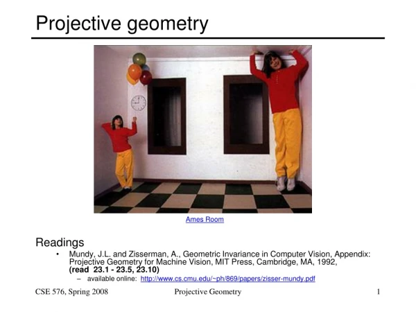
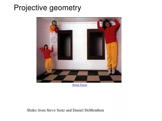
Projective geometry Ames Room
Projective geometry—what’s it good for? • Uses of projective geometry • Drawing • Measurements • Mathematics for projection • Undistorting images • Focus of expansion • Camera pose estimation, match move • Object recognition
Euclidean and Projective Geometry • Euclidean: they way things are • rigid body transformations • preserves, lengths, angles, parallel lines • Projective: the way they look • models how images of the 3D world appear • distorts angles, line lengths, parallelism
Applications of projective geometry Vermeer’s Music Lesson Reconstructions by Criminisi et al.
4 3 2 1 1 2 3 4 Measurements on planes Approach: unwarp then measure What kind of warp is this?
Image rectification p’ p • To unwarp (rectify) an image • solve for homography H given p and p’ • solve equations of the form: wp’ = Hp • linear in unknowns: w and coefficients of H • H is defined up to an arbitrary scale factor • how many points are necessary to solve for H? work out on board
(x,y,1) image plane The projective plane • Why do we need homogeneous coordinates? • represent points at infinity, homographies, perspective projection, multi-view relationships • What is the geometric intuition? • a point in the image is a ray in projective space -y (sx,sy,s) (0,0,0) x -z • Each point(x,y) on the plane is represented by a ray(sx,sy,s) • all points on the ray are equivalent: (x, y, 1) (sx, sy, s)
A line is a plane of rays through origin • all rays (x,y,z) satisfying: ax + by + cz = 0 l p • A line is also represented as a homogeneous 3-vector l Projective lines • What does a line in the image correspond to in projective space?
l1 p l l2 Point and line duality • A line l is a homogeneous 3-vector • It is to every point (ray) p on the line: lp=0 p2 p1 • What is the line l spanned by rays p1 and p2 ? • l is to p1 and p2 l = p1p2 • l is the plane normal • What is the intersection of two lines l1 and l2 ? • p is to l1 and l2 p = l1l2 • Points and lines are dual in projective space • given any formula, can switch the meanings of points and lines to get another formula
(a,b,0) -y -z image plane x • Ideal line • l (a, b, 0) • Corresponds to a line in the image (finite coordinates) • goes through image origin (principle point) Ideal points and lines • Ideal points (“points at infinity”) • p (x, y, 0) • intersection of parallel lines • infiniteimage coordinates • on the “line at infinity” (0,0,w) -y (sx,sy,0) x -z image plane
Homographies of points and lines • Given a homography on 3x3 matrix multiplication • transform a point: p’ = Hp • How do we need to adjust the line? • transform a line: lp=0 l’p’=0 • 0 =lp= (what goes here?) Hp= lH-1Hp =lH-1p’ l’ = lH-1 • Summary: lines are transformed bypost-multiplication of H-1
3D projective geometry • These concepts generalize naturally to 3D • Homogeneous coordinates • Projective 3D points have four coords: P = (X,Y,Z,W) • Duality • A plane N is also represented by a 4-vector • Points and planes are dual in 3D: N P=0 • Points at infinity (X,Y,Z,0) • intersection of 3D parallel lines • on the plane at infinity • imaged in 2D as vanishing points
vanishing point Vanishing points (2D) image plane • Vanishing point • projection of a point at infinity camera center ground plane
vanishing point Vanishing points (3D) image plane camera center line on ground plane
line on ground plane Vanishing points image plane • Properties • Any two 3D parallel lines have the same vanishing point v • The ray from C through v is parallel to the lines • An image may have more than one vanishing point • in fact every pixel is a potential vanishing point vanishing point V camera center C line on ground plane
v1 v2 Vanishing lines • Multiple Vanishing Points • Any set of parallel lines on the plane define a vanishing point • The union of all of these vanishing points is the horizon line • also called vanishing line • Note that different planes define different vanishing lines
Vanishing lines • Multiple Vanishing Points • Any set of parallel lines on the plane define a vanishing point • The union of all of these vanishing points is the horizon line • also called vanishing line • Note that different planes define different vanishing lines
Computing vanishing points V P0 D
Computing vanishing points • Properties • Pis a point at infinity, v is its projection • They depend only on line direction • Parallel lines P0 + tD, P1 + tDintersect at P V P0 D
Least squares version • Better to use more than two lines and compute the “closest” point of intersection • See notes by Bob Collins for one good way of doing this: • http://www-2.cs.cmu.edu/~ph/869/www/notes/vanishing.txt Computing vanishing points (from lines) • Intersect p1q1 with p2q2 v q2 q1 p2 p1
Vanishing line properties • Properties • l is intersection of horizontal plane through C with image plane • Compute l from two sets of parallel lines on ground plane • All points at same height as C project to l • points higher than C project above l • Provides way of comparing height of objects in the scene C l ground plane
Comparing heights Vanishing Point
Measuring height 5.4 5 Camera height 4 3.3 3 2.8 2 1
Epipolar geometry X x x’ • Baseline – line connecting the two camera centers • Epipolar Plane – plane containing baseline (1D family) • Epipoles • = intersections of baseline with image planes • = projections of the other camera center
The Epipole Photo by Frank Dellaert
Epipolar geometry X x x’ • Baseline – line connecting the two camera centers • Epipolar Plane – plane containing baseline (1D family) • Epipoles • = intersections of baseline with image planes • = projections of the other camera center • Epipolar Lines - intersections of epipolar plane with image planes (always come in corresponding pairs)
Example: Forward motion e’ e Epipole has same coordinates in both images. Points move along lines radiating from e: “Focus of expansion”
Epipolar constraint X • If we observe a point x in one image, where can the corresponding point x’ be in the other image? x x’
Epipolar constraint X X X x x’ x’ x’ • Potential matches for x have to lie on the corresponding • epipolar line l’. • Potential matches for x’ have to lie on the corresponding • epipolar line l.
Epipolar constraint: Calibrated case X • Assume that the intrinsic and extrinsic parameters of the cameras are known • We can multiply the projection matrix of each camera (and the image points) by the inverse of the calibration matrix to get normalized image coordinates • We can also set the global coordinate system to the coordinate system of the first camera x x’
Epipolar constraint: Calibrated case X = RX’ + t x x’ t R The vectors x, t, and Rx’ are coplanar
Epipolar constraint: Calibrated case X x x’ Essential Matrix (Longuet-Higgins, 1981) The vectors x, t, and Rx’ are coplanar
Epipolar constraint: Calibrated case X • E x’ is the epipolar line associated with x’(l = E x’) • ETx is the epipolar line associated with x (l’ = ETx) • E e’= 0 and ETe = 0 • E is singular (rank two) • E has five degrees of freedom x x’
Epipolar constraint: Uncalibrated case X • The calibration matrices K and K’ of the two cameras are unknown • We can write the epipolar constraint in terms of unknown normalized coordinates: x x’
Epipolar constraint: Uncalibrated case X x x’ Fundamental Matrix (Faugeras and Luong, 1992)