Download
1 / 63
640 likes | 746 Views
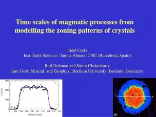
Time scales of magmatic processes from modelling the zoning patterns of crystals. Fidel Costa Inst. Earth Sciences ‘Jaume Almera’ CSIC (Barcelona, Spain) Ralf Dohmen and Sumit Chakraborty Inst. Geol. Mineral. and Geophys., Bochum University (Bochum, Germany). Table of contents.

E N D
Time scales of magmatic processes from modelling the zoning patterns of crystals Fidel CostaInst. Earth Sciences ‘Jaume Almera’ CSIC (Barcelona, Spain)Ralf Dohmen and Sumit ChakrabortyInst. Geol. Mineral. and Geophys., Bochum University (Bochum, Germany)
Table of contents 1. Introduction to zoning in crystals 2. Diffusion equation 3. Diffusion coefficient 4. Modeling natural crystals: isothermal case * Initial conditions * Boundary conditions • 5. Problems, pitfalls and uncertainities • * Multiple dimensions, sectioning, anisotropy • 6. Conclusions and prospects
X-ray distribution map of olivine from lava lake in Hawaii Moore & Evans (1967) Development of electron microprobe 1960’, first traverses and X-ray Maps Among the first applications to obtain time scales those related to cooling histories of meteorites (e.g. Goldstein and Short, 1967)
1. Zoning in crystals - Major elements, trace elements, and isotopes - Increasingly easier to measure gradients with good precision and spatial resolution (LA-ICP-MS, SIMS, NanoSIMS, FIB-ATEM, e-probe, micro-FTIR)
Major and trace element zoning in Plag
Stable isotope zoning 18O in zircon from Yellowstone magmas Bindeman et al. (2008)
Sr isotope zoning in plagioclase Tepley et al. (2000)
tt, Tt, Pt, Xt 1. Zoning in crystals Diffusion driven by a change in P, T, or composition t0, T0, P0, X0 concentration concentration distance distance
1. Zoning in crystals - The compositional zoning will reequilibrate at a rate governed by the chemical diffusion (Fick’s laws) - Because D is Exp dependent on T and Ds in geological materials are slow, minerals record high T events (as opposed to room T) distance
1. Zoning in crystals Crystals record the changes in variables and environments: gradients are a combined record of crystal growth and diffusion
2. Diffusion, flux, and Fick’s law Diffusion: (1) motion of one or more particles of a system relative to other particles (Onsager, 1945) (2) It occurs in all materials at all times at temperatures above the absolute zero (3) The existence of a driving force or concentration gradient is not necessary for diffusion
2. Diffusion, flux, and Fick’s law GAS LIQUID SOLID
Fick’s first law Flux has units of ‘mass or moles or volume * distance/time’ Diffusion coefficient has units of ‘distance2/time’ 2. Diffusion, flux, and Fick’s law Random motion leads to a net mass flux when the concentration is not uniform: equalizing concentration is a consequence, NOT the cause of diffusion
There might be other contribution to fluxes; e.g., crystal growth or dissolution 2. Diffusion, flux, and Fick’s law More general formulation by Onsager (1945) using the chemical potential
2. Diffusion, flux, and Fick’s law Fick’s second law: mass balance of fluxes Analogy: gain or loss in your bank account per month = Your salary ($$ per month) - what you spend ($$ per month)
2. Diffusion, flux, and Fick’s law Fick’s second law: mass balance of fluxes 1. We need to solve the partial differential diffusion equation. (a) analytical solution (e.g., Crank, 1975) or (b) numerical methods (e.g., Appendix I of chapter) 2. We need to know initial and boundary conditions. This is straightforward for ‘exercise cases’, less so in nature. 3. We need to know the diffusion coefficient
Di*= tracer diffusion coefficient w = frequency of a jump to an adjacent site l = distance of the jump f = related to symmetry, coordination number 3. Diffusion coefficient: Tracer e.g., diffusion of 56Fe in homogenous olivine
Multicomponent formulation (Lasaga, 1979) for ideal system, elements with the same charge and exchanging in the same site e.g., diffusion of FeMg olivine 3. Diffusion coefficient: multicomponent
Q = activation energy (at 105 Pa), ΔV =activation volume, P = pressure in Pascals, R is the gas constant, and Do = pre-exponential factor. 3. Diffusion coefficient Perform experiments at controlled conditions to determine D* or DFeMg
3. Diffusion coefficient New experimental and analytical techniques allow to determine D at the conditions (P, T, fO2, ai) relevant for the magmatic processes without need to extrapolation e.g., Fe-Mg in olivine along [001] Dohmen and Chakraborty (2007)
PLEASE CHECK APPENDIX II OF THE CHAPTER and AGU Oral presentation, Tuesday 8h30’ 3. Diffusion coefficient New theoretical developments allow a deeper understanding of the diffusion mechanism and thus to establish the extend to which experimentally determined D apply to nature (e.g., impurities, dislocations, etc).
4. Solving the diffusion equation Initial and boundary distribution (conditions)
4. Initial distribution (conditions) 4 strategies for initial distribution Shape of profile may retain info about initial distribution
Initial conditions 1. Use slower diffusing elements to constrain shape of faster elements • Examples • An for Mg in plagioclase (Costa et al., 2003) • P for Fe-Mg in olivine (Kahl et al., 2008) • Ba for Sr in sanidine (Morgan and Blake, 2006)
X-Ray Map of P Initial conditions 1. Use slower diffusing elements to constrain shape of faster elements OLIVINE Examples • Examples • An for Mg in plagioclase (Costa et al., 2003) • P for Fe-Mg in olivine (Kahl et al., 2008) • Ba for Sr in sanidine (Morgan and Blake, 2006) X-Ray Map of Fe
Initial conditions 2. Using arbitrary maximum initial concentration range in natural samples (this provides maximum time estimates) Examples * Sr in plagioclase (Zellmer et al., 1999) * Fe-Mg in Cpx (Costa and Streck, 2003; Morgan et al., 2006) * Ti in Qtz (Wark et al., 2007)
Initial conditions 3. Using a homogeneous concentration profile Examples * Fe-Mg, Ca, Ni, Mn in olivine (Costa and Chakraborty, 2004; Costa and Dungan, 2005) * O in zircon (Bindeman and Valley, 2001)
Initial conditions 4. Use a thermodynamic (e.g., MELTS) and kinetic model to generate a growth zoning profile Examples * Plagioclase (Loomis, 1982) * olivine- Chapter and AGU Poster, Tuesday afternoon
Initial conditions Conc. 100 Equil % Conc. 0 time distance
Initial conditions: effects on time scales 1. Despite the difference in shapes of the initial profiles the maximum difference on calculated time scales is a factor of ~1.5 2. Although the initial profile that we assume controls the time that we obtain, the error can be evaluated and is typically not very large 3. When in doubt perform models with different initial conditions to asses the range of time scales
X-Ray Map of Fe Open: the crystal exchanges with the surrounding (e.g., Fe-Mg in melt-olivine interface) Boundary conditions Characterizes the nature of exchange of the elements at the boundaries of the crystals (e.g., other crystals or melt). Two end-member possibilities
(a) D of the element of interest is much slower in the surrounding than in the mineral X-Ray Map of Ca Olivine e.g., Ca in olivine-plag contact Plag Boundary conditions 2. Closed: no exchange.
Boundary conditions 2. Closed: no exchange. (b) the mineral is surrounded by a phase where the element does not partition (e.g. Fe-Mg: olivine/plag) X-Ray Map of Mg Olivine Plag Kahl et al. (2008)
Boundary conditions Open boundary Conc. 100 Equil % Conc. 0 Closed boundary time distance
Boundary conditions: effects on time scales Equilibration in the closed system occurred much faster Incorrectly applying a no flux condition to an open system can lead to underestimation of time by factors as large as an order of magnitude. But in general not difficult to recognise which type of boundary applies to the natural situation
(b) Neglecting crystal dissolution tends to underestimate time scales (e.g., shortening of diffusion profiles) t1 Conc. distance t2 Conc. distance Boundary conditions: effects of crystal growth or dissolution (a) Neglecting crystal growth tends to overestimate time scales
Non-isothermal process * If there is no overall cooling of heating trend, results from a single intermediate T are correct, likely for some volcanic rocks (e.g., Lasaga and Jiang, 1995)
CHECK PAGES 13-21 of the CHAPTER AGU POSTER, 13h40’, Tuesday, Non-isothermal process * If there are protracted cooling and reheating (e.g., plutonic rocks) we need to have a T-t path *This affects: (a) the diffusion coefficient, (b) the diffusion equation, and (c) the boundary conditions.
Errors and uncertainties associated with time determinations Two types: (1) those associated with how well we understand and reproduce the natural physical conditions (e.g., multiple dimension etc), and (2) those associated with the parameters used in the model (e.g., T, D)
Off core sections; 2D effects on sectioning X-Ray Map of Mg X-Ray Map of Mg Kahl et al. (2008) Effects of geometry and multiple dimensions These are important depending on the type, shape, and size of the crystal that we are studying and on the diffusion time
Careful with the orientation of the diffusion front with respect to the traverse- one can create unnecessary and artificial 2D effects Not OK OK Effects of geometry and multiple dimensions Data acquisition Neglecting multidimensional effects tends to overestimate time scales
Example of plagioclase 1D, t = 225 y ini calc Costa et al (2003), GCA 67 equi Effects of geometry and multiple dimensions
ini calc Effects of geometry and multiple dimensions 1D, t = 225 y ------> 2D, t = 60 y almost a factor of 4!
c Model b Initial Fo zoning Mg zoning 150 µm Fe-Mg zoning in olivine: diffusion anisotropy and 2 dimensional effects
Anisotropy of diffusion EBSD Dt6 ?? Dt6 ~ Da T6: , , ?? ~0, ~, ~