Download
1 / 12
120 likes | 198 Views
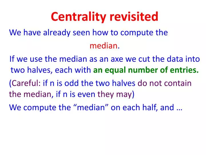
Centrality revisited We have already seen how to compute the median . If we use the median as an axe we cut the data into two halves, each with an equal number of entries. ( Careful: if n is odd the two halves do not contain the median , if n is even they may )

E N D
Centrality revisited We have already seen how to compute the median. If we use the median as an axe we cut the data into two halves, each with an equal number of entries. (Careful: if n is odd the two halves do not contain the median, if n is even they may) We compute the “median” on each half, and …
call the two resulting numbers (one on the left, one on the right of the median) the lower (on the left) quartile and the upper (on the right) quartile. We get this nice “breakdown of data:” That justifies the name quartiles (duh!) We could go on cutting sets of data in half, but not now. Instead we look at
Measures of “Spread” One measure of spread comes immediately to mind, the range, but a quick look at some examples shows right away that this isn’t precise enough, wildly different sets of data have the same range. Now what? Another way to look at spread, besides range (which is too crude a measure), is to look at how “spread out” the data are, that is, how far they wonder away from the middle.
Unfortunately we have to decide first which middle? Say we have a finite set of data x1, x2, x3, …, xn Intuitively we would like to take the median, but for computational ease we’ll choose the average, ( for a sample, for a population). So … we write the distance between and xifor each datum, add the distances and divide by n. We can write a long hand formula for this as follows:
Or an even prettier short hand formula (BUT forget about pretty long or pretty short, learn the method!) This is very nice, except that absolute values are computationally intractable! Much nicer (computationally)
The right-hand side is called the variance (denoted by Var) So we have the baptism (definition) (This formula may lead to fairly difficult computations, we’ll learn a short-cut soon) If the data are from the entire population of interest life is good. If however the data are from just a sample of the population, it turns out that
the value we get from Var tends to underestimate the true value of Var (from the entire population, such is life!) We compensate for this slight underestimation by a slight increase in the value of Var. We just multiply by the fraction (why is this an increase ?). In summary: populationVar sampleVar = (populationVar)•
We have stated before that the formula can lead to some seriously difficult computations. Try applying it to the set of numbers 3 5 7 -4 6 8 -2 There is, however, a short-cut. In formula it looks worse, but in words (and use) it is much easier.
In words it says: • First compute the mean • Then compute the mean of the squares 3. Then subtract 12 from 2. Let's try the short-cut on the set of numbers 3 5 7 -4 6 8 -2
Step 12 gives Step 2 gives We get Var =
When the number of data is small there is an even easier (visually) way to proceed. We apply it to the same set of seven data:
Final Remarks The variance we have computed is a population variance If the data come from a sample we must remember to correct our answer, multiplying by the correction factor Then we take a square root and obtain the corresponding standard deviation (population or sample)