Download

1 / 15
150 likes | 369 Views
Module 27 : Two Sample t-tests With Unequal Variances. This module shows how to test the hypothesis that two population means are equal when there is evidence that the requirement that the two populations have the same variance is not met. REVIEWED 19 July 05 /MODULE 27. The General Situation.

E N D
Module 27: Two Sample t-tests With Unequal Variances This module shows how to test the hypothesis that two population means are equal when there is evidence that the requirement that the two populations have the same variance is not met. REVIEWED 19 July 05 /MODULE 27
The General Situation Earlier we tested hypotheses about two population means, based on data from two independent samples under the assumption that the two populations had the same variance. For this situation, we calculated the pooled estimate of the common variance with:
We then tested the null hypothesis: H0 : µ1=µ2vs. H1: µ1 ≠ µ2 with the test statistic:
What if σ12≠ σ22 If the two population variances are not the same, then they are estimated separately and: is estimated by:
When we have two independent random samples from two different populations and there is evidence that the two population variances differ, i.e. 12 ≠ 22, then we can base a test about the difference between the population means 1 and 2 on the following:
To deal with 12 ≠ 22, we are adjusting the degrees of freedom in order to obtain a better approximation than would otherwise be the case. This adjustment requires that we calculate:
Example Independent random samples were taken from populations of histidine levels for males and females. The measurements were approximately normally distributed . The statistics from the two samples were:
Test the hypothesis H0: M = F vs. H1: M F • The hypothesis: H0: M = F vs H1: M F • The assumptions: Independent samples, normal distributions • The - level: = 0.05 • 4. The test statistic:
The critical region: Reject if t is not between t0.975(f), where • so that f = 6.99-2 = 4.99. We will use f = 5, and t0.975(5) = 2.57058.
6. The result: 7. The conclusion: The value calculated for t above is very close to the cut point so that P 0.05
Example: Am J Public Health, 1999;Dec:1692 Table 1 in the article by Sargent JD et al provides data on blood lead levels for samples from two communities. Test the hypothesis that Test the hypothesis that Test the hypothesis that