Download
1 / 48
480 likes | 652 Views
Spatiotemporal Networks in Addressable Excitable Media International Workshop on Bio-Inspired Complex Networks in Science and Technology Max Planck Institute for the Physics of Complex Systems Dresden, Germany, 5 - 9 May 2008. Co-Workers: Mark Tinsley Aaron Steel. Funding: NSF ONR

E N D
Spatiotemporal Networks in Addressable Excitable Media International Workshop on Bio-Inspired Complex Networks in Science and Technology Max Planck Institute for the Physics of Complex Systems Dresden, Germany, 5 - 9 May 2008 Co-Workers: Mark Tinsley Aaron Steel Funding: NSF ONR W.M. Keck Foundation
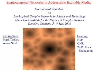
Photosensitive BZ Network Dark system is oscillatory. Excitability of medium maintained by reference light intensity. Medium is divided into an array of cells. Non-diffusive jumps from one cell to another (random) cell. Nearest-neighbor interactions described by reaction-diffusion wave. Long range interactions described by non-diffusive jumps. Phys. Rev. Lett. 95, 038306 (2005) Chaos 16, 015110 (2006)
Static Link Network 50 50 Local links occur via reaction-diffusion wave. Non-local links occur via reduction of light intensity at destination cell once a source cell reaches threshold. Threshold: 50% excited.
Network Architecture Mean path length: the average minimum separation of two nodes within the network. Clustering coefficient: the average number of links between neighbors of an individual node divided by the total possible number of links between these neighbors. Small and large number of links: values reflect the lattice and random graph. Intermediate number links: values typical of small-world networks.
Static Network with 10 Links Oregonator Model Simulations Successive snapshots from left to right Grid: 1000 × 1000 Cells: 20 × 20 grid pts 50 × 50 = 2500 cells Threshold: 50% excited
Static Networks: Links 100 Links 500 Links 10 links
Experimental Static Network with 300 Links Photo BZ experiment Successive snapshots at 15 s intervals Grid: 260 × 260 Cells: 10 × 10 grid pts 26 × 26 = 676 cells Threshold: 50% excited
Time Series of Fractional Coverage (a) Experiments: 26 × 26 node network with 300 nonlocal links (red) and 20 nonlocal links (blue). (b) Simulations: 50×50 node network with 200 nonlocal links (red)and 10 nonlocal links (blue).
Time of Travel Shading indicates time of travel from central node to a given node.
Weighted Shortest Distance Between Nodes Local links Nonlocal links Each local link is weighted as 1. Each nonlocal link is weighted as w. We use a shortest path algorithm to calculate the distance between nodes in the network (Dijkstra’s Algorithm). The distance between A and B is either 4 (nonlocal links) or 2+ w. C The weight w is chosen as the time necessary to initiate a nonlocal excitation in the BZ system. (w = nonlocal initiation time/local initiation time.) Typically w = 0.4.
Comparison of Network Distance and Time of Travel Model System: 50 x 50 nodes – 100 links short long fast slow Distance Time of travel Shading of each node indicates the shortest distance between that node and the central node. Shading of each node indicates time of travel of BZ wave to that node from the central node.
Comparison of Network Distance and Time of Travel BZ Experiment: 26 x 26 nodes – 10 links short long fast slow Distance Time of travel Shading of each node indicates the shortest distance between that node and the central node. Shading of each node indicates time of travel of BZ wave to that node from the central node.
Comparison of Network Distance and Time of Travel Model System: 50 x 50 nodes – 100 links short long fast slow Distance Time of travel Time of travel vs shortest distance indicates that the excitation propagates through the network via the shortest path between nodes. (Related to determination of optimal paths in a maze, since a maze is equivalent to a network of connected nodes.)
Frequency Synchronization 50 x 50 node network – 25 nodes shown
Distributed Network Pacemakers Excitation loops: links with destination nodes behind waves that excite the source nodes. Period defined by the time required for a wave to travel from the destination node to the source node plus the time for the nonlocal link to re-excite the destination node. Loop structure may have multiple local and nonlocal links. For few links: period of excitation loop is highly dependent on the network structure. For > 50 links: period is governed by the period of the excitation cycle. Error bars: standard deviation for 10 network configurations.
Phase Synchronization of Nodes R = normalized vector sum of the phases N = number of nodes θj = phase of the jth node. An R value close to zero indicates that the phases of the individual oscillators are evenly distributed, while an R value close to unity indicates the oscillators are in phase.
Active Links Pruning: a subset of links becomes inactive, while remaining active links account for dynamical behavior. Active link: nonlocal link that results in successful wave initiation at destination cell. Increasingly large spread in the values arises from increase in possible network configurations.
Stability of Active Link Sequence Sequence of active links: destination nodes are labeled according to the order of their excitations. Sequence of initiations is repeated once per coverage oscillation. Perturbation: (b) link 6 removed (c) link 4 removed from t = 24.4 to 40.0 Link sequence unstable to perturbation (b) while stable to perturbation (c).
Destination Node Locations of Active Links before and after Destabilizing Perturbation Original perturbation: destination node of link 6 ● Lost: destination node of links 4 ● and 6 ● Gained: destination nodes of links 15-19 ●
BZ Experiment: Pruning of Links Spontaneous shifting of active links during transient period as system relaxes to asymptotic sequence.
Network Architecture of Active Links Mean path length: the average minimum separation of two nodes within the network. Clustering coefficient: the average number of links between neighbors of an individual node divided by the total possible number of links between these neighbors. Active links have same scaling as random links. However, only 1/3 to 1/4 of the random links are active. Dynamics with 50 active links is approx. same as with 150 random links. Pruning results in network optimization.
Dynamic Network Successive snapshots from left to right. Grid: 1000×1000; Cells: 20 × 20 grid pts; Medium: 50×50 cells Jump threshold: 50% cell coverage; Jump probability: p = 0.02
Time Series and Power Spectrum Fraction of excited elements Jump probability p = 0.05
Time Series and Power Spectrum Fraction of excited elements Jump probability p = 0.4
Experimental Dynamic Link Network Photo BZ experiment Link probability p = 0.5 Successive snapshots at 15 s intervals Grid: 260 × 260 Cells: 10 × 10 grid pts 26 × 26 = 676 cells Threshold: 50% excited
Time Series and Power Spectra Dynamic link network with p = 0.01 (dotted line) and p = 0.50 (solid line). Coverage is the fraction of grid points in excited state. PSD is the power spectral density.
Domain Model Zipf Law for domain distribution. Links to any domain (other than domain of origin) with a fixed probability to random location in any other domain. Links from a domain proportional to departure domain size. Links to a domain ca. proportional to destination domain size (for large populations). Nearest neighbor interactions within a domain determine local spreading. Grid: 1000×1000 Cells: 10 × 10 grid pts Largest domain: 260 cells (population 2600)
Domains with Dynamic Links Jump probability p = 0.1
Domains with Dynamic Links Jump probability p = 0.3
Domains with Dynamic Links Jump probability p = 0.5
Time Series for Excitation Coverage p = 0.5 p = 0.3 p = 0.1 ←Collapse!
Domains with Dynamic Links Jump probability p = 0.5
Domains with Dynamic Links: Experiments Jump probability p = 0.05
Domains with Dynamic Links: Experiments Jump probability p = 0.7
Towards More Realistic Networks: Setting up the Links Neurons do not connect with other neurons randomly over a spatial domain. Neurons have a tendency to connect to nearby neurons and we approximate this tendency by an exponential falloff: P(d) = 1/ξ exp(-d/ξ) where P(d) is the connection probability at distance d, and ξ is the average connection distance parameter. H. Berry, and O. Temam, Lecture Notes in Computer Science, 3512:306-317, (2005)
Nature of Links: Integrate and Fire Neurons are activated according to an integrate and fire mechanism. In the context of the photo-BZ system, we have inputs to a node from all the connected nodes. The inputs are summed up and when they reach a threshold light intensity, the node fires (becomes excited). The destination node then becomes a source node with the excitation passed on according to the integrate and fire mechanism. We have assigned 20% of the links to be inhibitory.
Network Evolution without Diffusive Coupling Evolution of network activity without diffusive coupling: 1600 nodes and 125,000 links with 80% excitatory links (with weight of 0.03) and 20% inhibitory links (with weight of -0.08). Red represents excited state and blue represents steady state.
Network Evolution with Diffusive Coupling Evolution of network activity with diffusive coupling: 1600 nodes and 42,000 links with 80% excitatory links (with weight of 0.03) and 20% inhibitory links (with weight of -0.08). Red represents excited state and blue represents steady state.
Spike Timing-Dependent Plasticity (STDP) = • w represents the weight of a link, where • w → w + wp for potentiation. • w → w + wd for depression. M. Rossum, G. Bi & G. Turrigiano, “Stable Hebbian Learning from Spike Time-Dependent plasticity,” J. Neurosci. 20, 8812 (2000).
Application of STDP Active links affect a target cell, where wj is weight adjusted by changes wp or wd of link j based upon Δt.
Link Weight Distribution Distribution of link weights: 1600 nodes and 125,000 links with 80% excitatory links (initial weight of 0.03) and 20% inhibitory links (not shown, constant weight of -0.08). Excitatory link weight increases from 0.03 to and average of ~0.06 by STDP mechanism.
Weighted Degree Distribution Distribution of the sum of weighted links per node: Histogram shows number of nodes for each sum of weighted links. 1600 nodes and 125,000 links with 80% excitatory links (with initial weight of 0.03) and 20% inhibitory links (constant weight of -0.08).
Spatiotemporal Networks in Addressable Excitable Media Nearest neighbor spreading: Rxn-Diff wave Non-diffusive spreading: fixed random links Network distance and time of travel Frequency and phase synchronization Dynamic non-diffusive jumps and domain model Integrate and fire with inhibitory links Spike-timing dependent plasticity