Download
1 / 37
370 likes | 529 Views
Spatiotemporal Coordination in Wireless Sensor Networks. Dissertation Defense. Branislav Kusy branislav.kusy@gmail.com. Outline. Introduction What are wireless sensor networks? Contribution 1: Time Synchronization Structured design of time synchronization algorithms

E N D
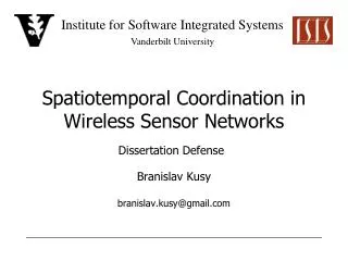
Spatiotemporal Coordination in Wireless Sensor Networks Dissertation Defense Branislav Kusy branislav.kusy@gmail.com
Outline • Introduction • What are wireless sensor networks? • Contribution 1: Time Synchronization • Structured design of time synchronization algorithms • Design and implementation of various time sync services • Contribution 2: Localization and Tracking • Radio interferometric ranging • Localization • Tracking
Wireless Sensor Networks (WSNs) scalability • cooperative networks of large size and high density
Wireless Sensor Networks (WSNs) scalability • cooperative networks of large size and high density • individual nodes: embedded, small size, low-power, cost resource efficiency
Wireless Sensor Networks (WSNs) scalability • cooperative networks of large size and high density • individual nodes: embedded, small size, low-power, cost • heterogeneity resource efficiency good hardware abstractions
Wireless Sensor Networks (WSNs) scalability • cooperative networks of large size and high density • individual nodes: embedded, small size, low-power, cost • heterogeneity • ad-hoc deployment resource efficiency good hardware abstractions self-configuration
Wireless Sensor Networks (WSNs) scalability • cooperative networks of large size and high density • individual nodes: embedded, small size, low-power, cost • heterogeneity • ad-hoc deployment • mobility resource efficiency good hardware abstractions self-configuration reconfiguration
Wireless Sensor Networks (WSNs) scalability • cooperative networks of large size and high density • individual nodes: embedded, small size, low-power, cost • heterogeneity • ad-hoc deployment • mobility • dynamically changing, inhospitable environments resource efficiency good hardware abstractions self-configuration reconfiguration autonomous operation failure recovery
Outline • Introduction • What are wireless sensor networks? • Contribution 1: Time Synchronization • Structured design of time synchronization algorithms • Design and implementation of various time sync services • Contribution 2: Localization and Tracking • Radio interferometric ranging • Localization • Tracking
Time Synchronization Challenges • large variety of time sync needs no method is optimal for all applications • heterogeneous and rapidly evolving hardware platforms new hardware platforms are introduced each year • high accuracy requirements but resource constrained hardware Time synchronization: a system service maintaining a common notion of time across multiple nodes over possibly multi-hop links 8-bit 7.37 MHz CPU 4kB RAM 56 kbps radio 2 AA batteries
Time Synchronization: Problem 1 Time synchronization algorithms are designed in an ad hoc way (for a specific platform or a specific application) time sync algorithm WSN application Problems • hardware is rapidly evolving • high accuracy requires detailed hardware understanding
Time Synchronization: Problem 1 Solution: design a hardware abstraction. time sync algorithm time sync algorithm WSN application hardware abstraction • shields time sync developers from hardware details • is the only piece of code that needs to be changed
Time Synchronization: Problem 2 WSN applications have different accuracy, power efficiency, or reliability needs. Hard to find the best matching time sync algorithm. • Solution • distill common time sync usage patterns from a set of WSN applications • standardize interfaces of the usage patterns • develop services that implement the interfaces • provide quantitative comparison of the services WSN applications TEST app SERVICE API SERVICE TEST app API SERVICE TEST app API SERVICE Application developers choose between time sync services rather than particular implementations! TEST app API
The Structured Approach to Time Synchronization We propose a three-layer architecture of time sync protocols. • One framework solves both problems • ETA time stamping primitive provides hardware abstraction • 3 time sync services identified
R2 R1 R3 S Hardware Abstraction Layer ETA (Elapsed Time on Arrival) • sender and receivers time stamp the message at the same instant (green) • sender includes his time stamp in the transmitted message (blue) time sync services send TS msg payload sync point ETA • synchronizes receiver to the sender • efficiency: single broadcast required • accuracy: a fewµs • implementation on different HW platforms: Mica2, Mica2dot, MicaZ, Telos, TelosB
Timesync Services Layer Event Timestamping Service • allows to convert event timestamps from the local times of the sensors to the base station local time Virtual Global Time Service • provides a single, shared, and continuously available global timebase Coordinated Action Service • allows to schedule a synchronized event in the future
event Tevent time node1 Δt1 time node2 Δt2 time node3 Δt3 time sink root Event Timestamping Service Routing Integrated Time Synchronization (RITS) • reactive protocol, synchronizes after the event was detected • maintains the age of event instead of the global time and computes the local time of event at the base station Pros • resource efficiency • virtually no communication overhead • Cons • clock skew is not compensated • large time sync errors if it takes long to route the messages Troot Δt1+ Δt2 + Δt3 Tevent = Troot - Δt1- Δt2 - Δt3
Event Timestamping Service Routing Integrated Time Synchronization (RITS) Evaluation • 45 Mica2 nodes deployed • software enforced neighbors • ~1000 simulated events Immediate routing Delayed routing 5.7 μs avg error 80 μs max error 34 μs avg error 297 μs max error
Centralized Virtual Global Time Rapid Time Synchronization Protocol (RaTS) • similar to RITS, the direction of messages is reversed • proactive protocol: periodic directed flooding from the root • clock skews are estimated at each node Pros • high accuracy • high tunability • Cons • central point of failure • timesyc msgs flooding 1 hour duty cycle Evaluation Low duty cycle (1 hour): 47 μs avg, 1.3ms max 20 sec convergence High duty cycle (30 sec): 2.7 μs avg, 26 μs max 4 sec convergence
Distributed Virtual Global Time Flooding Time Synchronization Protocol (FTSP) • distributed proactive protocol, no central point of failure • self-configuring, robust to link and node failures • periodic controlled flooding by each node Pros • high accuracy • fault tolerance • Cons • convergence time Evaluation Normal operation: 3 μs avg, 14 μs max Frequent failures: 17 μs avg, 67μs max Convergence: 14 min Duty cycle: 30 sec
Outline • Introduction • What are wireless sensor networks? • Contribution 1: Time Synchronization • Structured design of time synchronization algorithms • Design and implementation of various time sync services • Contribution 2: Localization and Tracking • Radio interferometric ranging • Localization • Tracking
Localization, Tracking, and Challenges Localization a system service that establishes spatial relations between nodes Tracking a system service that determines the location and velocity of mobile nodes continuously over time Challenges • high accuracy vs. resource constrained hardware • non-line of sight (NLOS) problems • different environments may require different methods No existing algorithm satisfies all three following criteria • high accuracy • long range • low cost (preferably no extra hardware cost)
Designing Novel Ranging Algorithm Objective: high accuracy, long range, and low cost ranging method Observation: utilizing the radio chips used for communication adds no extra cost Previous work: RSSI ranging RX power TX power 1. determine signal attenuation from TX power/RX power • 2. Use a Path Loss Model • 3. Calculate distance dist Transmitter Receiver Problems Radio signal amplitude is subject to variations due to channel noise, multipath fading, and interference coming from the environment. Extensive calibration is required, but RSSI is still imprecise beyond a few meters.
Designing Novel Ranging Algorithm • Utilize phase difference of arrival? TX phase 1. Transmit pure sine wave • 2. Find the TX and RX phase • 3. Calculate distance modulo wavelength λ RX phase RX TX dist λ Problems • COTS radio chips don’t provide control over TX phase • impossible to measure the phase of the high frequency radio signal (400 MHz) • very accurate timesync required (light travels 30cm in 1 ns which is 50% of λ)
Designing Novel Ranging Algorithm Two transmitters? Two receivers? RX1 RX1 phase f1≠f2 freq f2 TX dist1 dist2 dist1 Subtract the two distances and the TX phase falls out. Low frequency beat signal can be analyzed. Important result: phase of the beat signal equals phase difference of 2 original signals. dist2 freq f1 RX2 phase RX2 Problems • COTS radio chips don’t provide control over TX phase • impossible to measure the phase of the high frequency radio signal (400 MHz) • very accurate timesync required (light travels 30cm in 1 ns which is 50% of λ)
Radio Interferometric Ranging Use two transmitters and two receivers !!! • transmitters simultaneously transmit at slightly different frequencies • receivers measure the phase of the interference signal φCD= (dAD-dBD+dBC-dAC)mod λ interferometric range (q-range) • infinitely many solutions, in general • measure phase offsets at multiple carrier frequencies φ1CD = (dAD-dBD+dBC-dAC) modλ1 ... φkCD = (dAD-dBD+dBC-dAC) modλk
Radio Interferometric Localization How do we find node locations from q-ranges? Existing localization algorithms use trilateration/triangulation to find initial location estimates and then iteratively optimize locations using redundant data. trilateration triangulation No such method exists for q-ranges (dAD-dBD+dBC-dAC ). • Centralized genetic algorithm (GA) solution • given is a set of nodes with unknown locations and a set of measured q-ranges • starting with random locations, GA iteratively finds relative locations that best-fit the measured q-ranges • GA mutation operator translates, rotates, or scales one or multiple nodes
Evaluation of GA Localization • High accuracy • Long range • $0 extra HW cost • deployment parameters • 12000 m2 area • 16 XSM motes • 3 anchor nodes • 35m avg neighbor dist. • maximum range • 170m max • localization error • <4 cm avg • 12 cm max • took 50 minutes (!)
C D A B Radio Interferometric Tracking • Tracking • determine location and velocity of possibly mobile objects, continuously over time • we assume that some kind of tracking infrastructure is deployed Localization vs. tracking measurements • localization: q-range involves transmitters A and B, and receivers C and D qABCD = dAD-dBD+dBC-dAC • tracking: consider only measurements where B,C,D nodes are anchors and rearrange equation keeping the unknowns on the left side dAD-dAC =qABCD+dBD-dBC (qABCD is measured,dBD anddBC are given) • the new equation defines a hyperbola in 2D t-range q-range hyperbola
Calculating Locations in Tracking • Location estimation • node location is found at the intersection of hyperbolae Evaluation • Test at the football stadium • Vanderbilt football stadium • 12 infrastructure nodes • 80 x 90 m area • 0.6m avg and 1.5m max 2D error • single tracked node only • 3 sec update rate • hyperbolae intersect at a single point • except for the measurement error • search for a region which gets intersected by many hyperbolae
Calculating Velocity in Tracking Doppler effect: if the observer of a signal moves relative to the signal source, the perceived frequency of the signal is Doppler shifted Doppler effect in the context of interferometric tracking • two transmitters – only T is moving • the beat frequency measured at node Si is • relative speed vi of tracked node T can be calculated from the measured beat signal at Si • velocity v of the tracked node T is determined from the speeds vi using the location of T • Evaluation • similar experiment at the football stadium • 0.2 m/s speed, 11.5 degree orientation accuracy v
Tracking with RF Doppler Shifts Only • Can we track using only Doppler shifts? • find both location and velocity of target T from the relative speeds • advantages: measurements are simpler and faster • disadvantages: mobility is required • Approach • model location and velocity estimation as a non-linear optimization problem • parameters are x=(x,y,vx,vy,f^) • constraints are c=(f1,…,fn), beat frequencies measured by S1,…Sn • objective function F(x)=c v We developed CNLS-EKF algorithm that combines Constrained Non-linear Least Squares (CNLS) and Extended Kalman Filter (EKF) techniques.
CNLS-EKF Algorithm Evaluation We show that CNLS-EKF algorithm significantly improves EKF tracking accuracy in the maneuvering case, while keeping the good performance in the non-maneuvering case. • Evaluation • Vanderbilt football stadium • 50 x 30 m area • 9 infrastructure XSM nodes • 1 XSM mote tracked • position fix in 1.5 seconds maneuvering case Non-
Conclusions and Future Work • Time synchronization • We have introduced a structured approach to the design of time synchronization algorithms that allows for high synchronization accuracy and seamless code portability on a variety of hardware platforms. • Future work • design and implement other important time sync services • explore alternative timestamping primitives (ETA may not always be an option) • Localization • We have developed a novel interferometric ranging method which allows to achieve high accuracy, long range, and low cost simultaneously and built a number of localization and tracking algorithms on top of this ranging primitive. • Future work • utilize RSSI, phase offsets, and Doppler shifts in beat frequency measured at a single frequency • improve initialization and enable localization of stationary nodes
The End Thanks for the attention! Questions and Comments?
Solving the Optimization Problem • Non-linear Least Squares (NLS) and Extended Kalman Filter (EKF) • for our optimization problem, NLS often introduced significant errors (Fig. 1) • EKF improves tracking accuracy, but fails in the maneuvering case (Fig. 2) • resolved these problems by combining EKF and constrained NLS Figure 2 Figure 1