Download
1 / 23
230 likes | 488 Views
High latitude, deep, and thermohaline circulation. October 15. Rossby Number. Ratio of Advective Accelerations to Coriolis Advective Accel: u d u/dx; Coriolis: fu Ratio: (U 2 /L)/fU Define Rossby Number: R o = U/fL Where U=velocity scale L=length scale f= Coriolis parameter

E N D
High latitude, deep, and thermohaline circulation October 15
Rossby Number Ratio of Advective Accelerations to Coriolis Advective Accel: u du/dx; Coriolis: fu Ratio: (U2/L)/fU Define Rossby Number: Ro = U/fL Where U=velocity scale L=length scale f= Coriolis parameter If U=1m/s, L=100km, f=10-4 Then Ro= 0.1 <<1, so Coriolis (Geostrophy) dominates
heating cooling Thermohaline circulation Eq 80N CLASSICAL MODEL ONLY
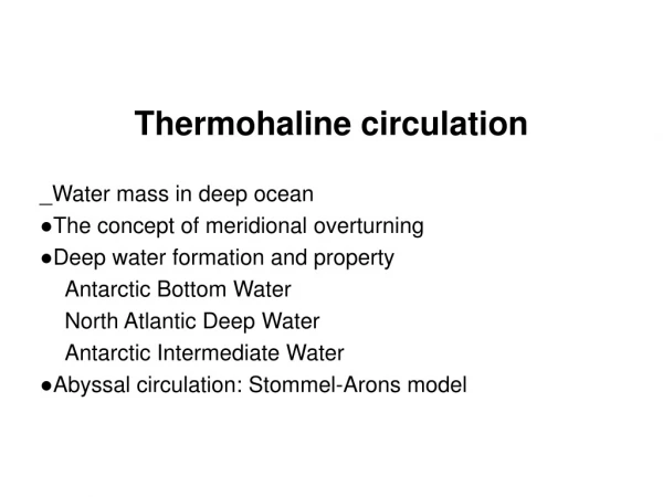
Thermohaline circulation • Result of the differential heating and cooling, and freshening and “salting” • i.e. dilution and concentration of salt in the ocean • Cooling occurs at poles, heat at (near) the equator • Cooling water sinks to the bottom – heated water stays in surface layer. Flows to the poles to replace sinking water. Cool water flows along the bottom and upwells towards low latitudes. • Also known as “Meridional Overturning Circulation”
Thermohaline circulation • Most of northward, warm water flow is through the mid-latitude western boundary current because surface flow elsewhere (wind-driven) is southward. • Also β-effect would tend to concentrate thermohaline circulation on west side of the ocean • Helps support western boundary currents
Importance of Deep Circulation • The contrast between the cold deep water and the warm surface waters determines the stratification of the oceans. Stratification strongly influences ocean dynamics. • The volume of deep water is far larger than the volume of surface water. Although currents in the deep ocean are relatively weak, they have transports comparable to the surface transports. • The deep circulation influences Earth's heat budget and climate. It varies on time scales from decades to centuries to millennia, and this variability is thought to modulate climate over such time intervals. The ocean may be the primary cause of variability over times ranging from years to decades, and it may have helped modulate ice-age climate.
Oceanic Transport of Heat • The oceans carry about half the heat from the tropics to high latitudes required to maintain Earth's temperature. Heat carried by the Gulf Stream and the north Atlantic drift warms Europe. Norway, at 60°N is far warmer than southern Greenland or northern Labrador at the same latitude. Palm trees grow on the west coast of Ireland, but not in Newfoundland which is farther south. • Global Conveyor Belt - The basic idea is that the Gulf Stream carries heat to the far north Atlantic. There the surface water releases heat and water to the atmosphere and the water becomes sufficiently dense that it sinks to the bottom in the Norwegian and Greenland Seas. The deep water later upwells in other regions and in other oceans, and eventually makes its way back to the Gulf Stream and the north Atlantic.
Figure 13.1 in Stewart. The surface (red, orange, yellow) and deep (violet, blue, green) currents in the North Atlantic. The North Atlantic Current brings warm water northward where it cools. Some sinks and returns southward as a cold, deep, western-boundary current. Some returns southward at the surface. From Woods Hole Oceanographic Institution.
Role of the Ocean in Ice-Age Climate Fluctuations • What might happen when the production of deep water in the Atlantic is shut off? Information contained in the Greenland and Antarctic ice sheets and in north Atlantic sediments provide important clues.
Figure 13.2 in Stewart. Periodic surges of icebergs during the last ice age appear to have modulated temperatures of the northern hemisphere by lowering the salinity of the far north Atlantic and reducing the meridional overturning circulation. Data from cores through the Greenland ice sheet (1), deep-sea sediments (2,3), and alpine-lake sediments (4) indicate that: Left: During recent times the circulation has been stable, and the polar front which separates warm and cold water masses has allowed warm water to penetrate beyond Norway. Center: During the last ice age, periodic surges of icebergs reduced salinity and reduced the Meridional Overturning Circulation, causing the polar front to move southward and keeping warm water south of Spain. Right: Similar fluctuations during the last interglacial appear to have caused rapid, large changes in climate. The Bottom plot is a rough indication of temperature in the region, but the scales are not the same.
The switching on and off of the meridional overturning circulation has large hysteresis (Figure 13.3 in Stewart). The circulation has two stable states. The first is the present circulation (1). In the second, (3) deep water is produced mostly near Antarctica, and upwelling occurs in the far north Pacific (as it does today) and in the far north Atlantic. Once the circulation is shut off, the system switches to the second stable state. The return to normal salinity does not cause the circulation to turn on. Surface waters must become saltier than average for the first state to return
Theory for the Deep Circulation • To describe the simplest aspects of the flow, we begin with the Sverdrup equation applied to a bottom current of thickness H in an ocean of constant depth: • Integrating this equation from the bottom of the ocean to the top of the abyssal circulation layer gives: V is the vertical integral of the northward velocity, and W0 is the velocity at the base of the thermocline: z=H – Note: z=0 at bottom!
Figure 13.4 in Stewart. Sketch of the deep circulation resulting from deep convection in the Atlantic (dark circles) and upwelling through the thermocline elsewhere. After Stommel (1958).
Figure 13.5 in Stewart. Sketch of the deep circulation in the Indian Ocean inferred from the temperature, given in °C. Note that the flow is constrained by the deep mid-ocean ridge system. After Tchernia (1980).
Observations of Deep circulation • Water masses • T-S plots are used to delineate water masses and their geographical distribution, to describe mixing among water masses, and to infer motion of water in the deep ocean. • water properties, such as temperature and salinity, are formed only when the water is at the surface or in the mixed layer. Heating, cooling, rain, and evaporation all contribute there. • Once the water sinks below the mixed layer, temperature and salinity can change only by mixing with adjacent water masses. Thus water from a particular region has a particular temperature associated with a particular salinity, and the relationship changes little as the water moves through the deep ocean.
Figure 13.6 in Stewart. Temperature and salinity measured at hydrographic stations on either side of the Gulf Stream. Data are from tables 10.2 and 10.4. Left: Temperature and salinity plotted as a function of depth. Right: The same data, but salinity is plotted as a function of temperature in a T-S plot. Notice that temperature and salinity are uniquely related below the mixed layer. A few depths are noted next to data points.
Figure 13.7 in Stewart Upper: Mixing of two water masses produces a line on a T-S plot. Lower: Mixing among three water masses produces intersecting lines on a T-S plot, and the apex at the intersection is rounded by further mixing. From Tolmazin (1985).
Figure 13.8 in Stewart. Mixing of two water types of the same density (L and G) produces water that is denser (M) than either water type. From Tolmazin (1985).
Figure 13.9 in Stewart. T-S plot of data collected at various latitudes in the western basins of the south Atlantic. Lines drawn through data from 5°N, showing possible mixing between water masses: NADW – North Atlantic Deep Water, AIW – Antarctic Intermediate Water, AAB - Antarctic Bottom Water, U - Subtropical Lower Water
Table 13.1 in Stewart. Water Masses of the South Atlantic between 33° S and 11° N
Figure 13.10 in Stewart. Contour plot of salinity as a function of depth in the western basins of the Atlantic from the Arctic Ocean to Antarctica. The plot clearly shows extensive cores, one at depths near 1000 m extending from 50°S to 20°N, the other at is at depths near 2000m extending from 20°N to 50°S. The upper is the Antarctic Intermediate Water, the lower is the North Atlantic Deep Water. The arrows mark the assumed direction of the flow in the cores. The Antarctic Bottom Water fills the deepest levels from 50°S to 30°N. See also Figures 10.16 and 6.11. From Lynn and Reid (1968).
Figure 13.11 in Stewart. T-S plots of water in the various ocean basins. From Tolmazin (1985).
Antarctic Circumpolar Current Figure 13.12 in Stewart. Cross section of neutral density across the Antarctic Circumpolar Current in the Drake Passage from the World Ocean Circulation Experiment section A21 in 1990. The current has three streams associated with the three fronts (dark shading): sACCf = Southern ACC Front, PF = Polar Front, and SAF = Subantarctic Front. Hydrographic station numbers are given at the top, and transports are relative to 3,000 dbar. Circumpolar deep water is indicated by light shading. From Orsi (2000).