Download
1 / 52
530 likes | 786 Views
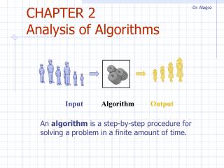
Analysis of Algorithms Lecture 2. Input. Output. Algorithm. Outline. Running time Pseudo-code Counting primitive operations Asymptotic notation Asymptotic analysis. How good is Insertion-Sort?. How can you answer such questions?. What is “goodness”?. Correctness

E N D
Analysis of AlgorithmsLecture 2 Input Output Algorithm
Outline • Running time • Pseudo-code • Counting primitive operations • Asymptotic notation • Asymptotic analysis Analysis of Algorithms
How good is Insertion-Sort? • How can you answer such questions? Analysis of Algorithms
What is “goodness”? • Correctness • Minimum use of “time” + “space” • Measure • Count • Estimate How can we quantify it? Analysis of Algorithms
1) Measure it – do an experiment! • Write a program implementing the algorithm • Run the program with inputs of varying size and composition • Use a method like System.currentTimeMillis() to get an accurate measure of the actual running time • Plot the results Analysis of Algorithms
Limitations of Experiments • Must implement the algorithm, which may be difficult! • Results may not reflect the running time on other inputs • In order to compare two algorithms, the same hardware and software environments must be used Analysis of Algorithms
2) Count Primitive Operations • The Idea • Write down the pseudocode • Count the number of “primitive operations” Analysis of Algorithms
Example: find max element of an array AlgorithmarrayMax(A, n) Inputarray A of n integers Outputmaximum element of A currentMaxA[0] fori1ton 1do ifA[i] currentMaxthen currentMaxA[i] returncurrentMax Pseudocode • High-level description of an algorithm • More structured than English prose • Less detailed than a program • Preferred notation for describing algorithms • Hides program design issues Analysis of Algorithms
Control flow if…then… [else…] while…do… repeat…until… for…do… Indentation replaces braces Method declaration Algorithm method (arg [, arg…]) Input… Output… Method call var.method (arg [, arg…]) Return value returnexpression Expressions Assignment(like in Java) Equality testing(like in Java) n2 Superscripts and other mathematical formatting allowed Pseudocode Details Analysis of Algorithms
2 1 0 The Random Access Machine (RAM) Model • A CPU • An potentially unbounded bank of memory cells, each of which can hold an arbitrary number or character • Memory cells are numbered and accessing any cell in memory takes unit time. Analysis of Algorithms
Random Access Model (RAM) • Time complexity (running time) = number of instructions executed • Space complexity = the number of memory cells accessed Analysis of Algorithms
Basic computations performed by an algorithm Identifiable in pseudocode Largely independent from the programming language Exact definition not important (we will see why later) Examples: Evaluating an expression Assigning a value to a variable Indexing into an array Calling a method Returning from a method Primitive Operations Analysis of Algorithms
Analyzing pseudocode (by counting) • For each line of pseudocode, count the number of primitive operations in it. Pay attention to the word "primitive" here; sorting an array is not a primitive operation. • Multiply this count with the number of times this line is executed. • Sum up over all lines. Analysis of Algorithms
By inspecting the pseudocode, we can determine the maximum number of primitive operations executed by an algorithm, as a function of the input size AlgorithmarrayMax(A, n) Cost Times currentMaxA[0] 2 1 fori1ton 1do 2 n ifA[i] currentMaxthen 2 (n 1) currentMaxA[i] 2 (n 1) { increment counter i } 2 (n 1) returncurrentMax1 1 Total8n3 operations Counting Primitive Operations Analysis of Algorithms
Algorithm arrayMax executes 8n3 primitive operations in the worst case Define a Time taken by the fastest primitive operation b Time taken by the slowest primitive operation Let T(n) be the actual worst-case running time of arrayMax. We havea (8n3) T(n)b(8n3) Hence, the running time T(n) is bounded by two linear functions Estimating Running Time Analysis of Algorithms
Insertion Sort • Hint: • observe each line i can be implemented using a constant number of RAM instructions, Ci • for each value of j in the outer loop, we let tj be the number of times that the while loop test in line 4 is executed. Analysis of Algorithms
Insertion Sort Question: So what is the running time? Analysis of Algorithms
Time Complexity may depend on the input! • Best Case:? • Worst Case:? • Average Case:? Analysis of Algorithms
Complexity may depend on the input! • Best Case: Already sorted. tj=1. Running time = C * N (a linear function of N) • Worst Case: Inverse order. tj=j. Analysis of Algorithms
Neglecting the constants, the worst-base running time of insertion sort is proportional to1 + 2 + …+ n The sum of the first n integers is n(n+ 1) / 2 Thus, algorithm insertion sort required almost n2 operations. Arithmetic Progression Analysis of Algorithms
What about the Average Case? • Idea: • Assume that each of the n! permutations of A is equally likely. • Compute the average over all possible different inputs of length N. • Difficult to compute! • In this course we focus on Worst Case Analysis! Analysis of Algorithms
See TimeComplexity Spreadsheet Analysis of Algorithms
Analysis of AlgorithmsLecture 3 Input Output Algorithm
What is “goodness”? • Correctness • Minimum use of “time” + “space” • Measure wall clock time • Count operations • Estimate Computational Complexity How can we quantify it? Analysis of Algorithms
Asymptotic Analysis • Uses a high-level description of the algorithm instead of an implementation • Allows us to evaluate the speed of an algorithm independent of the hardware/software environment • Estimate the growth rate of T(n) • A back of the envelope calculation!!! Analysis of Algorithms
The idea • Write down an algorithm • Using Pseudocode • In terms of a set of primitive operations • Count the # of steps • In terms of primitive operations • Considering worst case input • Bound or “estimate” the running time • Ignore constant factors • Bound fundamental running time Analysis of Algorithms
Growth Rate of Running Time • Changing the hardware/ software environment • Affects T(n) by a constant factor, but • Does not alter the growth rate of T(n) • The linear growth rate of the running time T(n) is an intrinsic property of algorithm arrayMax Analysis of Algorithms
Which growth rate is best? • T(n) = 1000n + n2 or T(n) = 2n + n3 Analysis of Algorithms
Growth Rates • Growth rates of functions: • Linear n • Quadratic n2 • Cubic n3 • In a log-log chart, the slope of the line corresponds to the growth rate of the function Analysis of Algorithms
Functions Graphed Using “Normal” Scale g(n) = n lg n g(n) = 1 g(n) = n2 g(n) = lg n g(n) = n g(n) = 2n g(n) = n3 Analysis of Algorithms
Constant Factors • The growth rate is not affected by • constant factors or • lower-order terms • Examples • 102n+105is a linear function • 105n2+ 108nis a quadratic function Analysis of Algorithms
Big-Oh Notation • Given functions f(n) and g(n), we say that f(n) is O(g(n))if there are positive constantsc and n0 such that f(n)cg(n) for n n0 • Example: 2n+10 is O(n) • 2n+10cn • (c 2) n 10 • n 10/(c 2) • Pick c = 3 and n0 = 10 Analysis of Algorithms
f(n) is O(g(n)) iff f(n)cg(n) for n n0 Analysis of Algorithms
Big-Oh Notation (cont.) • Example: the function n2is not O(n) • n2cn • n c • The above inequality cannot be satisfied since c must be a constant Analysis of Algorithms
More Big-Oh Examples • 7n-2 7n-2 is O(n) need c > 0 and n0 1 such that 7n-2 c•n for n n0 this is true for c = 7 and n0 = 1 • 3n3 + 20n2 + 5 3n3 + 20n2 + 5 is O(n3) need c > 0 and n0 1 such that 3n3 + 20n2 + 5 c•n3 for n n0 this is true for c = 4 and n0 = 21 • 3 log n + 5 3 log n + 5 is O(log n) need c > 0 and n0 1 such that 3 log n + 5 c•log n for n n0 this is true for c = 8 and n0 = 2 Analysis of Algorithms
Big-Oh and Growth Rate • The big-Oh notation gives an upper bound on the growth rate of a function • The statement “f(n) is O(g(n))” means that the growth rate of f(n) is no more than the growth rate of g(n) • We can use the big-Oh notation to rank functions according to their growth rate Analysis of Algorithms
Questions • Is T(n) = 9n4 + 876n = O(n4)? • Is T(n) = 9n4 + 876n = O(n3)? • Is T(n) = 9n4 + 876n = O(n27)? • T(n) = n2 + 100n = O(?) • T(n) = 3n + 32n3 + 767249999n2 = O(?) Analysis of Algorithms
Big-Oh Rules (shortcuts) • If is f(n) a polynomial of degree d, then f(n) is O(nd), i.e., • Drop lower-order terms • Drop constant factors • Use the smallest possible class of functions • Say “2n is O(n)”instead of “2n is O(n2)” • Use the simplest expression of the class • Say “3n+5 is O(n)”instead of “3n+5 is O(3n)” Analysis of Algorithms
Rank From Fast to Slow… • T(n) = O(n4) • T(n) = O(n log n) • T(n) = O(n2) • T(n) = O(n2 log n) • T(n) = O(n) • T(n) = O(2n) • T(n) = O(log n) • T(n) = O(n + 2n) Note: Assume base of log is 2 unless otherwise instructed i.e. log n = log2 n Analysis of Algorithms
Computing Prefix Averages • We further illustrate asymptotic analysis with two algorithms for prefix averages • The i-th prefix average of an array X is average of the first (i+ 1) elements of X A[i]= X[0] +X[1] +… +X[i] • Computing the array A of prefix averages of another array X has applications to financial analysis Analysis of Algorithms
Prefix Averages (Quadratic) • The following algorithm computes prefix averages in quadratic time by applying the definition AlgorithmprefixAverages1(X, n) Inputarray X of n integers Outputarray A of prefix averages of X #operations A new array of n integers n fori0ton 1do n sX[0] n forj1toido 1 + 2 + …+ (n 1) ss+X[j] 1 + 2 + …+ (n 1) A[i]s/(i+ 1)n returnA 1 Analysis of Algorithms
The running time of prefixAverages1 isO(1 + 2 + …+ n) The sum of the first n integers is n(n+ 1) / 2 There is a simple visual proof of this fact Thus, algorithm prefixAverages1 runs in O(n2) time Arithmetic Progression Analysis of Algorithms
Prefix Averages (Linear) • The following algorithm computes prefix averages in linear time by keeping a running sum AlgorithmprefixAverages2(X, n) Inputarray X of n integers Outputarray A of prefix averages of X #operations A new array of n integers n s 0 1 fori0ton 1do n ss+X[i] n A[i]s/(i+ 1)n returnA 1 • Algorithm prefixAverages2 runs in O(n) time Analysis of Algorithms
Math you may need to Review • Summations • Logarithms and Exponents • Proof techniques • Basic probability • properties of logarithms: logb(xy) = logbx + logby logb (x/y) = logbx - logby logbxa = alogbx logba = logxa/logxb • properties of exponentials: a(b+c) = aba c abc = (ab)c ab /ac = a(b-c) b = a logab bc = a c*logab Analysis of Algorithms
Big-Omega • Definition: f(n) is (g(n)) if there is a constant c > 0 and an integer constant n0 1 such that f(n) c•g(n) for n n0 • An asymptotic lower Bound Analysis of Algorithms
Big-Theta • Definition: f(n) is (g(n)) if there are constants c’ > 0 and c’’ > 0 and an integer constant n0 1 such that c’•g(n) f(n) c’’•g(n) for n n0 • Here we say that g(n) is an asymptotically tight bound for f(n). Analysis of Algorithms
Big-Theta (cont) • Based on the definitions, we have the following theorem: • f(n) = Θ(g(n)) if and only if f(n) = O(g(n)) and f(n) = Ω(g(n)). • For example, the statement n2/2 + lg n = Θ(n2) is equivalent to n2/2 + lg n = O(n2) and n2/2 + lg n = Ω(n2). • Note that asymptotic notation applies to asymptotically positive functions only, which are functions whose values are positive for all sufficiently large n. Analysis of Algorithms
Prove n2/2 + lg n = Θ(n2). • Proof. To prove this claim, we must determine positive constants c1, c2 and n0, s.t. c1 n2<= n2/2 + lg n <= c2 n2 • c1 <= ½ + (lg n) / n2 <= c2 (divide thru by n2) • Pick c1 = ¼ , c2 = ¾ and n0 = 2 • For n0 = 2, 1/4 <= ½ + (lg 2) / 4 <= ¾, TRUE • When n0 > 2, the (½ + (lg 2) / 4) term grows smaller but never less than ½, therefore n2/2 + lg n = Θ(n2). Analysis of Algorithms
Intuition for Asymptotic Notation Big-Oh • f(n) is O(g(n)) if f(n) is asymptotically less than or equal to g(n) big-Omega • f(n) is (g(n)) if f(n) is asymptotically greater than or equal to g(n) big-Theta • f(n) is (g(n)) if f(n) is asymptotically equal to g(n) Analysis of Algorithms