Polynomial Equivalent Layer
This paper presents a novel approach using Polynomial Equivalent Layer (PEL) techniques to transform potential field data for geophysical applications. The classical equivalent-layer technique encounters obstacles during large-scale inversions, which PEL addresses by utilizing a regular grid of equivalent-source windows. Within each window, the physical property distribution is characterized by a bivariate polynomial. This method enhances the estimation of the physical property distribution in both synthetic and real data applications, providing improved stability and accuracy in the resultant models.


Polynomial Equivalent Layer
E N D
Presentation Transcript
Polynomial Equivalent Layer Vanderlei C. Oliveira Jr Observatório Nacional Valéria C. F. Barbosa* Observatório Nacional
Contents • Classical equivalent-layer technique • The main obstacle • PolynomialEquivalentLayer(PEL) • Synthetic Data Application • Real Data Application • Conclusions
Equivalent-layer principle Potential-field observations produced by a 3D physical-property distribution can be exactly reproduced by a continuous and infinite 2D physical-property distribution Potential-field observations E N x y 3D sources Depth z
Equivalent-layer principle Potential-field observations produced by a 3D physical-property distribution can be exactly reproduced by a continuous and infinite 2D physical-property distribution Potential-field observations E N x y 2D physical-property distribution Depth z
Equivalent-layer principle This 2D physical-property distribution is approximated by a finite set of equivalent sources arrayed in a layer with finite horizontal dimensions and located below the observation surface Potential-field observations E N x y Equivalent sources may be magnetic dipoles, doublets, point masses. Layer of equivalent sources Equivalent Layer (Dampney, 1969). Depth z Equivalent sources
Equivalent-layer principle To perform any linear transformation of the potential-field data such as: • Interpolation (e.g., Cordell, 1992; Mendonça and Silva, 1994) • Upward (or downward) continuation (e.g., Emilia, 1973; Hansen and Miyazaki, 1984; Li and Oldenburg, 2010) • Reduction to the pole of magnetic data (e.g., Silva 1986; Leão and Silva, 1989; Guspí and Novara, 2009). • Noise-reduced estimates (e.g., Barnes and Lumley, 2011) How ?
Classical equivalent-layer technique
d N R Î Classical equivalent-layer technique We assume that the M equivalent sources are distributed in a regular grid with a constant depthzo forming an equivalent layer Potential-field observations E N x y Equivalent sources zo Equivalent Layer Depth
Classical equivalent-layer technique Why is it an obstacle to estimate the physical property distribution by using the classical equivalent-layer technique? How does the equivalent-layer technique work? Step 1: Step 2: Potential-field observations E E N N y x x y Transformed potential-field data ? Physical-property distribution p* = t T Depth Equivalent Layer Estimated physical-property distribution p*
Classical equivalent-layer technique A stable estimate of the physical properties p* is obtained by using: p* = (GT G+ m I ) -1GT d, Parameter-space formulation (M x M) (N x N) or p* = GT(GGT + m I ) -1d Data-space formulation The biggest obstacle A large-scale inversion is expected.
Objective We present a new fast method for performing any linear transformation of large potential-field data sets Polynomial Equivalent Layer (PEL)
Polynomial Equivalent Layer The equivalent layer is divided into a regular grid of Q equivalent-source windows Inside each window, the physical-property distribution is described by a bivariate polynomial of degreea. Q 2 1 Equivalent sources kth equivalent-source window with Msequivalent sources dipoles (in the case of magnetic data) point masses(in the case ofgravity data). Ms<<< M
Polynomial Equivalent Layer The physical-property distribution within the equivalent layer is assumed to be a piecewise polynomial function defined on a set of Q equivalent-source windows. Equivalent-source window Physical-property distribution Polynomial function
Polynomial Equivalent Layer How can we estimate the physical-property distribution within the entire equivalent layer ? Equivalent-source window Physical-property distribution
Polynomial Equivalent Layer k k k p c B Relationship between the physical-property distributionpkwithin the kth equivalent-source window and the polynomial coefficientsckof the ath-order polynomial function Polynomial coefficientsck Physical-property distribution pk kth equivalent-source window = Physical-property distribution
Polynomial Equivalent Layer é ù 1 B 0 0 L ê ú 2 0 B 0 L ê ú = Β ê ú M M O M ê ú Q ê ú 0 0 B L ë û How can we estimate the physical-property distribution pwithin the entire equivalent layer ? All polynomial coefficientsc Physical-property distribution p Q equivalent-source windows Entire equivalent layer p c B = (H x 1) (M x H) (M x 1) Physical-property distribution
Polynomial Equivalent Layer How does the Polynomial Equivalent Layer estimate c*? How does the Polynomial Equivalent Layer work? Step 1: Transformed potential-field data Step 3: t p* T = Potential-field observations E N E N Step 2: Physical-property distribution ? Equivalent layer with Q equivalent-source windows p* = c* B Estimated polynomial coefficients Computed physical-property distribution p* Depth c*
Polynomial Equivalent Layer T T B G d -1 [ ] ( ) + m m + m T T T T B G G B I B R R B 1 0 A stable estimate of the polynomial coefficients c* is obtained by * c = (H x H) A system of H linear equations in H unknowns H is the number of all polynomial coefficients describing all polynomial functions H <<<<M H <<<< N Polynomial Equivalent Layer requires much less computational effort
Polynomial Equivalent Layer THE CHOICES: • Size of the equivalent-source window • Degree of the polynomial A simple criterion is the following: The shorter the wavelength components of the anomaly the smaller the size of the equivalent-source window and the lower the degree of the polynomial should be.
Polynomial Equivalent Layer EXAMPLES Small-equivalent source window and Low degree of the polynomial (a = 1) Large-equivalent source window and High degree of the polynomial (a = 3) Gravity data set Magnetic data set
Polynomial Equivalent Layer Physical-property distribution How can we check if the choices of the size of the equivalent-source window and the degree of the polynomial were correctly done? Estimated physical-property distribution via PEL yields Unacceptable data fit. Acceptable data fit. A smaller size of the equivalent-source window and (or)anotherdegree of the polynomial must be tried.
Application of Polynomial Equivalent Layer (PEL) to synthetic magnetic data Reduction to the pole
Polynomial Equivalent Layer Simulated noise-corrupted total-field anomaly computed at 150 m height The geomagnetic field has inclination of -3o and declination of 45o. The magnetization vector has inclination of -2o and declination of -10o. The number of observations is about 70,000 A B C
Polynomial Equivalent Layer Two applications of Polynomial Equivalent Layer (PEL) First-order polynomials Large-equivalent-source window Small-equivalent-source window
First Application of Polynomial Equivalent Layer Large-equivalent-source windows and First-order polynomials M ~75,000equivalent sources The classical equivalent layer technique should solve 75,000 × 75,000 system H ~ 500 unknown polynomial coefficients The PEL solves a 500 × 500 system Large window
First Application of Polynomial Equivalent Layer Computed magnetization-intensity distribution obtained by PEL with first-order polynomials and large equivalent-source windows A/m
First Application of Polynomial Equivalent Layer Differences (color-scale map) between the simulated (black contour lines) and fitted (not show) total-field anomalies at z = -150 m. Poor data fit nT Large window
Second Application of Polynomial Equivalent Layer Small-equivalent-source windows and First-order polynomials M ~ 75,000 equivalent sources The classical equivalent layer technique should solve 75,000 × 75,000 system H ~ 1,900 unknown polynomial coefficients The PEL solves a 1,900 × 1,900 system Small window
Second Application of Polynomial Equivalent Layer Computed magnetization-intensity distribution obtained by PEL with first-order polynomials and small equivalent-source windows A/m
Second Application of Polynomial Equivalent Layer Differences (color-scale map) between the simulated (black contour lines) and fitted (not show) total-field anomalies at z = -150 m. Acceptable data fit. nT Small window
Polynomial Equivalent Layer True total-field anomaly at the pole (True transformed data)
Polynomial Equivalent Layer Reduced-to-the-pole anomaly (dashed white lines) using the Polynomial Equivalent Layer (PEL)
Application of Polynomial Equivalent Layer to real magnetic data Upward continuation and Reduction to the pole
Brazil São Paulo Aeromagnetic data set over the Goiás Magmatic Arc, Brazil. Rio de Janeiro
Real Test The geomagnetic field has inclination of -21.5o and declination of -19o. Small-equivalent-source windows and First-order polynomials The magnetization vector has inclination of -40o and declination of -19o. N ~ 78,000 observations Aeromagnetic data set over the Goiás Magmatic Arc in central Brazil. M ~ 81,000 equivalent sources The classical equivalent layer technique should solve 78,000 × 78,000 system H ~ 2,500 unknown polynomial coefficients The PEL solves a 2,500 × 2,500 system N Small-equivalent source window
Real Test N Computed magnetization-intensity distribution obtained by Polynomial Equivalent Layer (PEL)
Real Test N Observed (black lines and grayscale map) and predicted (dashed white lines) total-field anomalies. Acceptable data fit.
Real Test N Transformed data produced by applying the upward continuation and the reduction to the pole using the Polynomial Equivalent Layer (PEL)
Conclusions Polynomial Equivalent Layer We have presented a new fast method (Polynomial Equivalent Layer- PEL) for processing large sets of potential-field data using the equivalent-layer principle. The PEL divides the equivalent layer into a regular grid of equivalent-source windows, whose physical-property distributions are described by polynomials. The estimated polynomial-coefficients viaPEL are transformed into the physical-property distribution and thus any transformation of the data can be performed. ThePELsolves a linear system of equations with dimensions based on the total number H of polynomial coefficients within all equivalent-source windows, which is smaller than the number Nof data and the numberMof equivalent sources H <<<<< N H <<<<< M
Thank you for your attention Published in GEOPHYSICS, VOL. 78, NO. 1 (JANUARY-FEBRUARY 2013) 10.1190/GEO2012-0196.1