Download
1 / 26
440 likes | 1.59k Views
Chapter 4 Measures of Dispersion, Skewness and Kurtosis. I Range ( R ) A. Noninclusive Range. B. Inclusive Range. II Semi-Interquartile Range ( Q ). 1. Third quartile ( Q 3 ). 2. First quartile ( Q 1 ). Table 1. Taylor Manifest Anxiety Score. 74 1 73 1 72 0

E N D
Chapter 4 Measures of Dispersion, Skewness and Kurtosis I Range (R) A. Noninclusive Range B. Inclusive Range
II Semi-Interquartile Range (Q) 1. Third quartile (Q3) 2. First quartile (Q1)
Table 1. Taylor Manifest Anxiety Score 74 1 73 1 72 0 71 2 70 7 24 69 8 17 68 5 9 67 2 4 66 1 2 65 1 1 n = 28
III Another Median-like Statistic A. Percentile Point (P%)
IV Standard Deviation A. Sample Standard Deviation (S) B. Population Standard Deviation () where denotes the population mean
C. Standard Deviation Formula for Data in a Frequency Distribution 1. fj denotes the frequency in the jth class interval; Xj denotes the midpoint of the jth class interval.
Table 2. Taylor Manifest Anxiety Scores 74 1 74 1(23.5918) 73 1 73 1(14.8776) 72 0 0 0(8.1633) 71 2 142 2(3.4490) 70 7 490 7(0.7347) 69 8 552 8(0.0204) 68 5 340 5(1.3061) 67 2 134 2(4.5918) 66 1 66 1(9.8776) 65 1 65 1(17.1633) n = 28 1,936 93.4286
V Index of Dispersion (D) 1. DP = no. of distinguishable pairs of observations in c = 2 to k categories observations in c categories
B. Range of D is 0–1 1. D = 0 represents no dispersion (no distinguishable pairs); all n observations are in the same category 2. D = 1 represents maximum dispersion (observations are distributed equally over the c categories. 3. Example with c = 2 categories: category A represents one man (a1); category B represents five women (b1, . . . , b5)
4. (a) Observed data; (b) Example of maximum dispersion DP a1b1a1b2a1b3a1b4a1b5 DPmax a1b1a1b2a1b3a2b1a2b2a2b3a3b1a3b2a3b3
5. (a) Observed data; (b) Example of maximum dispersion DP a1b1a1b2a1b3a1b4a2b1 a2b2 a2b3 a2b4 DPmax a1b1a1b2a1b3a2b1a2b2a2b3a3b1a3b2a3b3
C. Alternative Computational Formula for D c = number of categories n = total number of observations nj= number of observations in the jth category
E. Computational Example with c = 5 Categories Table 3. Admission Data for Students Applied for Race Admission (AA) Admitted (A) n % n % White 268 82.2 179 78.9 Black 36 11.0 29 12.8 Mex/Amer. 16 4.9 18 7.9 Other 3 0.9 1 0.4 Unknown 3 0.9 0 0 n = 326 n = 227
1. Dispersion for students admitted is greater than that for students who applied for admission.
VI Relative Merits of the Four Measures of Dispersion VII Minimum and Maximum Values of S A. Maximum Value of S 1. Example using the Taylor Manifest Anxiety data in Table 2
2. For these data, R = 74.5 – 64.5 = 10 and n = 28. B. Minimum Value of S for Data in Table 2
IX Detecting Outliers A. Two Criteria Based on the Mean and Median (Taylor Manifest Data from Tables 1 & 2)
B. Criterion Based on a Box Plot 1. Left whisker computation 2. Right whisker computation
C. Box Plot 1. An asterisk (*) identifies one outlier
X Skewness (Sk) A. Interpretation of Sk Sk > 0, positively skewed Sk = 0, symmetrical Sk < 0, negatively skewed
B. Computational Example Table 4. Quiz Scores 2 –4 16 –64 256 4 –2 4 –8 16 7 1 1 1 1 8 2 4 8 16 9 3 9 27 81 30 0 34 –36 370 __________________________________________
1. Standard deviation for data in Table 4 2. Skewness for data in Table 4
XI Kurtosis (Kur) A. Interpretation of Kur Kur < 0, platykurtic Kur = 0, mesokurtic Kur < 0, leptokurtic