Download
1 / 24
250 likes | 318 Views
This comprehensive guide delves into the world of nonlinear optics, covering topics such as multiphoton excitation, inversion of CH3F molecules, and the Bloch vector model. Learn about harmonic generation, modulation of absorption, and dispersion effects. Discover the intricacies of short pulses, interactions with energy levels, and the manipulation of high-order Kerr refractive index. Delve into the density matrix and explore applications like climbing an anharmonic ladder of levels. This text is a valuable resource for those interested in the fascinating realm of nonlinear optics.

E N D
Coherent Nonlinear Optics 1. Nonlinear Optics 2. Romeo and Juliet Cascade multiphoton excitation 3. Application to the inversion of CH3F 4. From the cascade to the Bloch vector model Adiabatic approximation
From “Coherent Interactions” to “Nonlinear Optics” Bloch’s equations: near a resonance, time dependent population transfers, Modulation of the absorption and dispersion, resulting in a modulation of the pulse (effects: pulse reshaping, changes in spectrum around the pulse carrier frequency) Traditional nonlinear optics: creation of harmonics of the field because of a power expansion of the polarization: P = eo(ce + c(2)e2 + ... ) The nonlinearity is enhanced by a resonance. Procedure: calculate the expectation value of the dipole moment P = <y|m|y> For a two-level system at w0 perturbed by a field at w. Result: modified Bloch’s equations. What is the traditional nonlinear optics limit? Harmonic generation? How to have maximum efficiency?
of the order of 0.1 : pm/V Thus, to have 2) Estimate of Nonlinear optics and short pulses Limitations of the traditional approach P = P(E) 1) It is a Taylor series. A Taylor series has to converge A highly controversed example: V. Loriot, E. Hertz, O. Fauchet and B. Lavorel, "Measurement of high order Kerr refractive index of major air components", Optics Express, 17:13439—13434 (2009) (intensity required?) requires a field of the order of TV/m 2 solutions: either short pulse high intensity, or very high Q resonance (narrow bandwidth, long times) (long crystals, long propagation, dispersion problems, etc)
Nonlinear optics and short pulses Short pulse implies broad spectrum For linear polarization:
Nonlinear optics and short pulses Short pulse implies broad spectrum For linear polarization: It gets more complex for the next order: The Fourier transform of this correlation is also a correlation: If we introduce the Fourier transform of the nonlinear susceptibility:
Nonlinear optics and short pulses In the case of an instantaneous response: Inverse Fourier transform:
Nonlinear optics and short pulses Nonlinear optics involves generally interaction of a photon with a higher level of energy It is generally multiphoton with eventual intermediate near or exact resonances.
Nonlinear optics and short pulses In most cases involving a resonance of order n, with detuning , there will be a “driving vector”: and a “driven” vector representative of the atomic system, with components in quadrature with in phase with = energy stored in the atomic system The “equations of motion” will be that of a gyroscope - (relaxation)
TWO representations for nonlinear optics and short pulses Instead of A complex vector with components along real and imaginary axis, and and a complex
Interaction of light with a cascade of levels near resonance We will NOT start with a system having ONE near-resonance of order n, but with a cascade of n levels all near resonance. We will restrict ourselves to n = 3. Generalization to n > 3 is straightforward.
Interaction of light with a cascade of levels near resonance Rotating frame approximation:
Interaction of light with a cascade of levels near resonance This systems takes a simpler form is we define the Rabi frequencies as: Solve, and construct This is the density matrix the matrix
Interaction of light with a cascade of levels near resonance The approach presented here applies to different level systems. The different configurations of 3 level systems are: Two-photon resonant Interaction with resonant Intermediate level V-level systems L-level systems
CH3F Example of application: the ladder to heaven! Climbing an anharmonic ladder of levels
Example of application: the ladder to heaven! Climbing an anharmonic ladder of levels Solve, and construct 5 levels instead of 3 This is the density matrix the matrix Density matrix 5 x 5
1 0 0 0 0 0.45 x x x 0.89 0 0 0 0 0 0 0 0 0 0 x x x x x .1 0 0 0 0 0 0 0 0 0 x 0 0 0 0 0 0 0 0 0 0 0 0 0 0 0 0 0 0 0 -.1 0 0 0 0 0 0 0 0 0 0.89 x x x 0.44 0 0 0 0 0.94 Example of application: the ladder to heaven! Climbing an anharmonic ladder of levels 0.23 0.41 -0.2 0 time
1 0 0 0 0 0.45 x x x 0.89 0 0 0 0 0 0 0 0 0 0 x x x x x .1 0 0 0 0 0 0 0 0 0 x 0 0 0 0 0 0 0 0 0 0 0 0 0 0 0 0 0 0 0 -.1 0 0 0 0 0.89 x x x 0.44 0 0 0 0 0 0 0 0 0 0.94 Example of application: the ladder to heaven! Climbing an anharmonic ladder of levels Diels, Besnainou, J. Chem. Phys. 85: 6347 (1986) 0.23 0.41 -0.2 0 time
R branch: m = 1, 2, 3… Rotational levels: P branch: m = 1, 2, 3… are detuned by The levels labeled with quantum number Example of application: the ladder to heaven! There can be more steps to the ladder to heaven! Diels, Besnainou, J. Chem. Phys. 85: 6347 (1986) Instead of: Initial Boltzman distribution:
0.2 Level population 0.1 0 5 10 J Rotational quantum number Example of application: the ladder to heaven! There can be more steps to the ladder to heaven, but you get there anyway. Diels, Besnainou, J. Chem. Phys. 85: 6347 (1986)
Coherent Nonlinear Optics 1. Nonlinear Optics 2. Romeo and Juliet Cascade multiphoton excitation 3. Application to the inversion of CH3F 4. From the cascade to the Bloch vector model Adiabatic approximation
Adiabatic approximation Detuning of the intermediate level 1 larger than the transition rates: the second equation can be considered to be in steady state, and one can solve for the coefficient c1:
Adiabatic approximation Defining: Leads to:
Adiabatic approximation Bloch vector model
Adiabatic approximation Bloch vector model Contained in these expressions: Third order susceptibility, two-photon absorption, third harmonic generation, stimulated Raman, phase conjugated FWM, etc...