Nonlinear Optics: Phenomena, Materials and Devices
210 likes | 849 Views
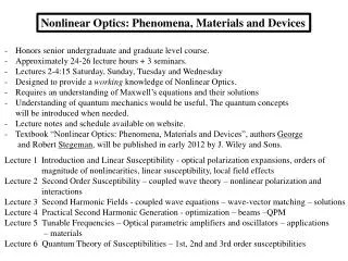
Nonlinear Optics: Phenomena, Materials and Devices. Honors senior undergraduate and graduate level course. Approximately 24-26 lecture hours + 3 seminars. Lectures 2-4:15 Saturday, Sunday, Tuesday and Wednesday Designed to provide a working knowledge of Nonlinear Optics.

Nonlinear Optics: Phenomena, Materials and Devices
E N D
Presentation Transcript
Nonlinear Optics: Phenomena, Materials and Devices • Honors senior undergraduate and graduate level course. • Approximately 24-26 lecture hours + 3 seminars. • Lectures 2-4:15 Saturday, Sunday, Tuesday and Wednesday • Designed to provide a working knowledge of Nonlinear Optics. • Requires an understanding of Maxwell’s equations and their solutions • Understanding of quantum mechanics would be useful, The quantum concepts • will be introduced when needed. • Lecture notes and schedule available on website. • Textbook “Nonlinear Optics: Phenomena, Materials and Devices”, authors George • and Robert Stegeman, will be published in early 2012 by J. Wiley and Sons. Lecture 1 Introduction and Linear Susceptibility - optical polarization expansions, orders of magnitude of nonlinearities, linear susceptibility, local field effects Lecture 2 Second Order Susceptibility – coupled wave theory – nonlinear polarization and interactions Lecture 3 Second Harmonic Fields - coupled wave equations – wave-vector matching – solutions Lecture 4 Practical Second Harmonic Generation - optimization – beams –QPM Lecture 5 Tunable Frequencies – Optical parametric amplifiers and oscillators – applications – materials Lecture 6 Quantum Theory of Susceptibilities – 1st, 2nd and 3rd order susceptibilities
Lecture 7 Nonlinear Index and Absorption – simple two & three level models – frequency dispersion – examples Lecture 8 Third Order Nonlinearities Due to Electronic Transitions: Materials – molecules - glasses – semiconductors Lecture 9 Miscellaneous (Slower) Third Order Nonlinearities: Materials -vibrational, electrostrictive, liquid crystal, electrostrictive, cascading effects Lecture 10 Ramifications and Applications of Nonlinear Refraction - self-focusing and defocusing - instabilities - solitons - bistability - all-optical switching Lecture 11 Multi-Wave Mixing - degenerate and non-degenerate four wave mixing – three wave mixing - nonlinear spectroscopy Lecture 12 Stimulated Scattering - stimulated Raman and Brillouinscattering Lecture 13 Extreme Nonlinear Optics - Ultra-Fast and Ultra-High Intensity Lecture 14 “Overflow” • Terminology • Fields written as • Superscript “roof” or “hat” (example ) emphasizes a complexquantity • The unit vector is written as and has components where i=x, y, z. • The “Einstein” notation is used for summations over repeated indices. • For example, • Quantities with a “bar” on top, e.g. refers to individual properties of isolated • molecules in a single molecule’s frame of reference. • - SI (mks) units are used throughout
Examples of Nonlinear Optics Examples of behavior associated with nonlinear optics Intensity dependent transmission Harmonic generation Nonlinear Interferometry Soliton generation and modulation instability Increasing input intensity
Classical Expansion of the Nonlinear Polarization The second order polarization is created at time t and position by two separate interactions of the total EM field with the medium at time and position , and at time and position in a material in which (2)0. This form includes nonlocality in space and time.
Frequency Spectrum Due to Non-Instantaneous Response e.g. 2 level system, excited state with lifetime ; excited with pulse t<< After passage of pulse Before incidence of pulse Evolution of frequency spectrum with time
Polarization Expansion: Nonlinearity Localized in Space Summation over all of the input frequencies present Note that all possible combinations of 1+2 are needed!
Magnitudes of Nonlinear Susceptibilities • Depends on the number of electrons in an atom (or molecule), distribution of • energy levels etc. • Consider hydrogen atom with one electron • will give a minimum value • analytical solutions known for energy, levels etc. The atomic Coulomb field binding the electron to the proton in its lowest orbit is Assume that the perturbation expansion for the nonlinear polarization is valid up to E 0.1Eatomic
Simple Model: Electron on a Spring (1) 2 ways to calculate the nonlinear susceptibilities Electron as an anharmonic oscillator – resonance frequencies are given by energy difference between ground and excited states simple but approximate Quantum mechanics – electric dipole transitions between atomic (molecular ) energy levels exact but complicated Electron on a Spring Model For 3D, need 3 springs with the spring displacements . The electron motion is that of a simple harmonic oscillator along these directions. The directions are chosen parallel to the axes which diagonalize the molecular polarizabilitytensor and hence . This does not imply that the higher order susceptibilities are diagonalized along these axes!
Field Induced Electron Displacement Simple Harmonic Oscillator Potential The spring constant is given in terms of the resonance frequencies by . The decay of the spring motion (lifetime of excited state) means that there is damping of the SHO and the driven SHO equation, with the electron charge, is given by Inertial force Spring restoring force Electromagnetic driving force
Local Field Effects (1) Maxwell’s equations in the material and the usual boundary conditions at the interface are valid for spatial averages of the fields over volume elements small on the scale of a wavelength, but large on the scale of a molecule. The “averaged” quantities also include the refractive index, the Poynting vector, and the so-called Maxwell field which has been written here as . It is the Maxwell field that satisfies the wave equation for a material with averaged refractive index n. At the site of a molecule the situation can be quite complex since the dipoles induced by the Maxwell electric fields on all the molecules create their own electric fields which must be added to the “averaged” field to get the total (“local”) field acting on a molecule. It is very difficult to calculate the “local” field accurately because it depends on crystal symmetry, intermolecular interactions, etc. Standard treatments like Lorenz-Lorenz are only approximately valid even for isotropic and cubic crystal media.
Local Field Effects (2) Dipole moments of the molecules induced by the Maxwell field produce a Maxwell polarization in the material. Consider a spherical cavity around the molecule of interest to find the local field acting on the molecule. Assuming that the effects of the induced dipoles inside the cavity average to zero, the polarization field outside the cavity induces charges on the walls of the cavity which produce an additional electric field on the molecule in the cavity. + + + + + + + + - + - + + - - - - - - - - -